In the recently released KFS report of 2021 – the National Forest Resources Assessment Report 2021 – Kenya has a tree cover of 7,180,600.66ha, which is 12.13% of the total area. Based on the national ambition to reach 10% tree cover by 2022, this is a monumental achievement. Forest cover, on the other hand, has a coverage of 5, 226, 197.79ha, a paltry 8.83% of the total area. Tree cover and forest cover are two terms that are sometimes used synonymously. However, they are different. Forest cover, as per the KFS report, refers to the amount of land area covered by a forest. Its counterpart terminology – tree cover, is a lit bit vaguer. Even FAO does not seem to have a commonly agreed definition. But for the purposes of this article, it refers to any area covered by trees, within or outside forests.
There has been a widespread assumption that each country should have a minimum of 10% forest cover, supposedly from an unconfirmed UN statement. An online search shows there has been, and still continues to be a debate on this threshold. This assumption arose from the definition of a ‘forest’ itself, in which, inter alia the ground under it must be under 15% or more canopy cover. A scholarly debate on this matter revealed it is better for countries to define their own optimum threshold. This is because each country has differing climate regimes, land availability and vegetation biomes. Thus, it best seems to leave countries to design their own fate on how much of their territory should be allocated to forest cover.
In Kenya, it is already engraved in stone. The constitution recommends at least 10% of the total area should be under forest cover.
Scholarly debates aside, we will try to corroborate, or rather, see if we can verify the findings of the KFS 2021 report on nothing else but through desktop research. We already know forest coverage is 8% of the total area, so we will check out if our remote sensing analysis comes close to this. If Eratosthenes of Cyrene was able to measure the circumference of the earth with reasonable accuracy with nothing more than mere trigonometry, surely we –2000 years down the line can do better armed with the latest software and tech. Can’t we?
To stop beating around the bush, we will use GEE, Qgis and Excel for forest cover assessment in the country. Let’s see if it comes close to the 8.83% mentioned in the report.
Are you ready to plunge in with both feet?
The Google Earth Engine
Like a time machine that can take you to, or back to different epochs of time, so is Google Earth Engine (GEE) in the geospatial world, minus the time travel. The Google Earth Engine (GEE) is a cloud computing platform designed to store and process huge data sets (at a petabyte-scale) for analysis and ultimate decision-making. Like in a time machine where one can input the date they would like to teleport to, GEE works in a similar way by providing a plethora of geospatial data – satellite images, vector datasets and curated algorithms to help the user investigate and discover various geographical phenomena for their place of interest. It has been especially useful to remote sensing scientists, ecologists, and even social researchers.
In this exercise, the Global PALSAR-2/PALSAR Forest/Non-Forest Map was used. Why this one? Basically for two reasons. It had a better spatial resolution than most. Secondly, it had the most recent coverage dating 2018-01-01. The Hansen Global Forest Change v1.9 (2000-2021) was a very tempting dataset to use, its recent coverage dates to 2021. However, it is beaten off the track in that its tree-cover data is for 2000, with the most recent statistics only showing tree loss for the last twenty years (2000 – 2021). 🙁
Armed with what we will swim, let’s take a deep dive.
Ready.
Set.
Dive.
The GEE Workflow
The entire workflow code, at least for the GEE part, is shown below.
//load the shapefile of Kenya
var Kenya = ee.FeatureCollection('USDOS/LSIB/2017')
    .filter(ee.Filter.eq('COUNTRY_NA', 'Kenya'));

//show the map of Kenya
Map.addLayer(Kenya, {}, 'Kenya');
Map.centerObject(Kenya, 7);

//so far so good

//load the global PALSAR dataset
var dataset = ee.ImageCollection('JAXA/ALOS/PALSAR/YEARLY/FNF')
    .filterDate('2017-01-01', '2017-12-31');

//check out the global PALSAR dataset
print("PALSAR dataset", dataset);

//show the global PALSAR dataset
Map.addLayer(dataset, {palette: ['green', 'yellow', 'blue'], min:1, max:3},
'PALSAR');

//green, yellow, blue colors represent the forest, non-forest and water bands
//of PALSAR respectively, as shown using min:1 and max:3 values, respectively

//so far so good

//show the Kenyan map above
Map.addLayer(Kenya, {}, 'Kenya');

//so far so good

//clip the global PALSAR dataset to Kenya only
//first show the forest class only
var forest = dataset.select('fnf')


//from this forest variable, choose value 1 which stands for trees
//lets first convert from image collection to image only. We will take the
//mean of 2017 as the forest cover
var forestonly = forest.mean();

//select values 1 which stand for forest from the forestonly image
var forestonly2 = forestonly.updateMask(forestonly.eq(1));

//add the forestonly image to see if non-forests have been masked out
Map.addLayer(forestonly2, {palette: ['green']}, 'Forest only');

//so far so good

//now time to clip to Kenya only
var kenyaForests = forestonly2.clip(Kenya);

//lets see forests in Kenya only
Map.addLayer(kenyaForests, {palette: ['green']}, 'Forests in Kenya');

//so far so good

// lets make these pixels of forests have an attribute of area, to help in
//calculations
print("Forest in Kenya", kenyaForests); //to get a feel of the data

var forestArea = kenyaForests.multiply(ee.Image.pixelArea());

print("Forests with area attribute", forestArea);

//the help says that the ee.Image.pixelArea() shall return a band
//called 'area'. However, our image, does not have this band 'area'.

//so far, so good, maybe

//calculate the area of forests in Kenya

var forestedArea = forestArea.reduceRegion({
  reducer: ee.Reducer.sum(),        //research more on reducers
  geometry: Kenya,         //the region to reduce data to or operating area
  scale: 10,           //the scale in meters to work in, went with Sentinel2
  crs: 'epsg:32737',   //used local projection WGS 84 UTM zone 37S
  bestEffort: true,   //used true so that server could determine its own best
  maxPixels: 1e7      //the default of 10000000
});

print("forestedArea", forestedArea);

//get total forested area in sq km
var forestKm = ee.Number(forestedArea.get('fnf')).divide(1e6);
print('Area of forests in sq kilometers: ', forestKm);

//get total forested area in ha
var forestHa = ee.Number(forestedArea.get('fnf')).divide(1e4);  //a ha = 10000sq. metres
print('Area of forests in hectares: ', forestHa);

//lets start phase 2
//load the counties dataset
Map.addLayer(counties, {}, 'Counties of Kenya');

//disaggregated the forestedArea statistics to each county

var countyForests = forestArea.reduceRegions({
  collection: counties,    //the uploaded counties shapefile
  reducer: ee.Reducer.sum(),  //calculate the sum area of forestedArea per county
  scale: 10,             //chose a resolution same as that of Sentinel 2
  crs: 'epsg:32737'     //used a local datum of WGS 84 Zone 37S
});

print('Area of forests in counties: ', countyForests);

//export the table of area of forests per county to google drive
Export.table.toDrive({
  collection: countyForests,    //the table with forest area statistics per county
  description: 'county_forestarea_metres', //the title of the table
  folder: 'test',   //the folder the table will be saved into
  fileFormat: 'CSV'
});

//view the forest coverage in counties
Map.addLayer(counties, {}, 'Counties');
And additionally, there was a county dataset which we will explain later.
var counties = Table users/sammigachuhi-test/counties_kenyaTime for a gasp of air. Let’s take this code out bit by bit.
Loading the Kenya shapefile to GEE
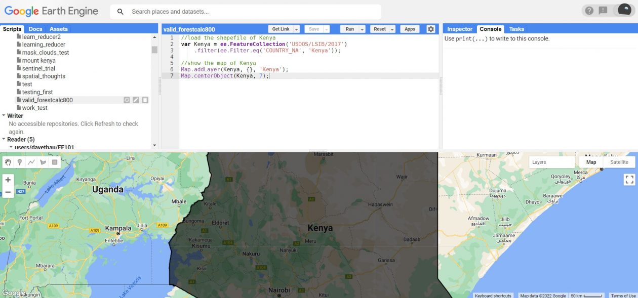
We will load the Kenya administrative shapefile into GEE. The purpose of this to delineate our focus area – the Area of Interest (AOI). Even though this should not necessarily be the first step, it helps (and pays) to start simple.
//load the shapefile of Kenya
var Kenya = ee.FeatureCollection('USDOS/LSIB/2017')
    .filter(ee.Filter.eq('COUNTRY_NA', 'Kenya'));

//show the map of Kenya
Map.addLayer(Kenya, {}, 'Kenya');
Map.centerObject(Kenya, 7);
So far so good.
You should see the map of Kenya on your GEE canvas.
Viewing the Global PALSAR data
Now that we have been able to define our AOI, we can take a step further and view the global PALSAR dataset. This will be like moving from sipping tea to taking the first bite of a cookie. Unlike loading the Kenya shapefile which was relatively straightforward, this one has some nuances.
//load the global PALSAR dataset
var dataset = ee.ImageCollection('JAXA/ALOS/PALSAR/YEARLY/FNF')
    .filterDate('2017-01-01', '2017-12-31');

//check out the global PALSAR dataset
print("PALSAR dataset", dataset);

//show the global PALSAR dataset
Map.addLayer(dataset, {palette: ['green', 'yellow', 'blue'], min:1, max:3},
'PALSAR');

//green, yellow, blue colors represent the forest, non-forest and water bands
//of PALSAR respectively, as shown using min:1 and max:3 values, respectively

//so far so good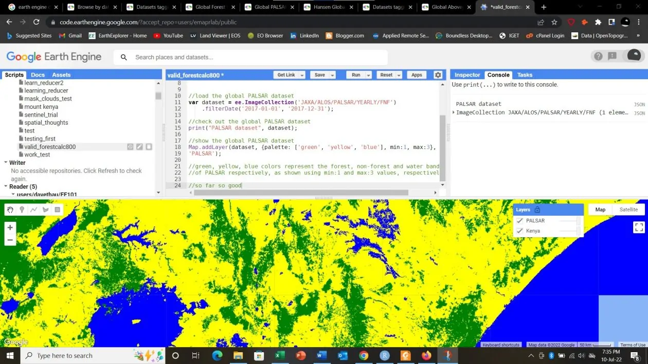
So far so good.
Notice that some new methods such as .filterDate, print() and Map.addLayer() were included in this code block. GEE has various methods for conducting geospatial analyses. The reader is advised to look them up.
Next, in order to have a feel of the forest cover in the country, we shall overlie the Kenya shapefile on top of the Global PALSAR dataset. This is why it was not necessary to load the Kenya shapefile in the first step. We could have loaded it here. However, we wanted to start simple, that’s why.
//show the Kenyan map above
Map.addLayer(Kenya, {}, 'Kenya');

//so far so good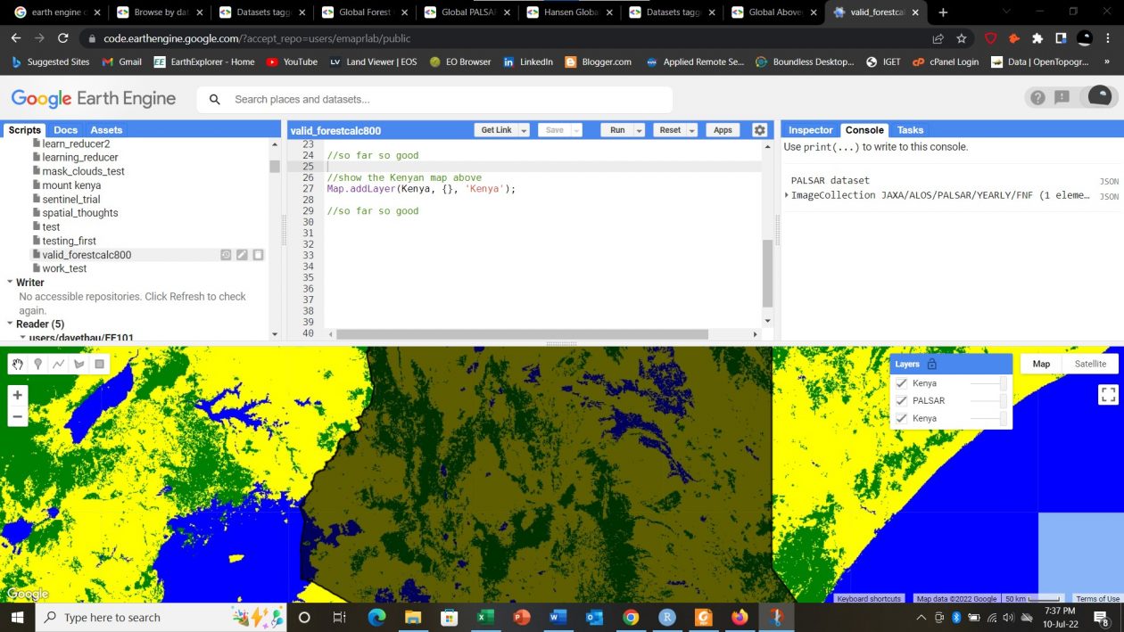
So far so good.
Mask out non-forest
Time to remove the unnecessary food items from our plates – the shell from the egg, and the peel from the fruit. In our case, let’s remain with forests only.
Already, if you are keen, you may have noted that some of the forest areas, which are green, and the waterbodies (in blue) are highly exaggerated. Since when did we have a water body the size of L. Albert, and a forest the size of Aberdares in North Eastern? Take note of this.
Let’s first remove the non-forested areas.
//first show the forest class only
var forest = dataset.select('fnf')

//from this forest variable, choose value 1 which stands for trees
//lets first convert from image collection to image only. We will take the
//mean of 2017 as the forest cover
var forestonly = forest.mean();

//select values 1 which stand for forest from the forestonly image
var forestonly2 = forestonly.updateMask(forestonly.eq(1));

//add the forestonly image to see if non-forests have been masked out
Map.addLayer(forestonly2, {palette: ['green']}, 'Forest only');

//so far so good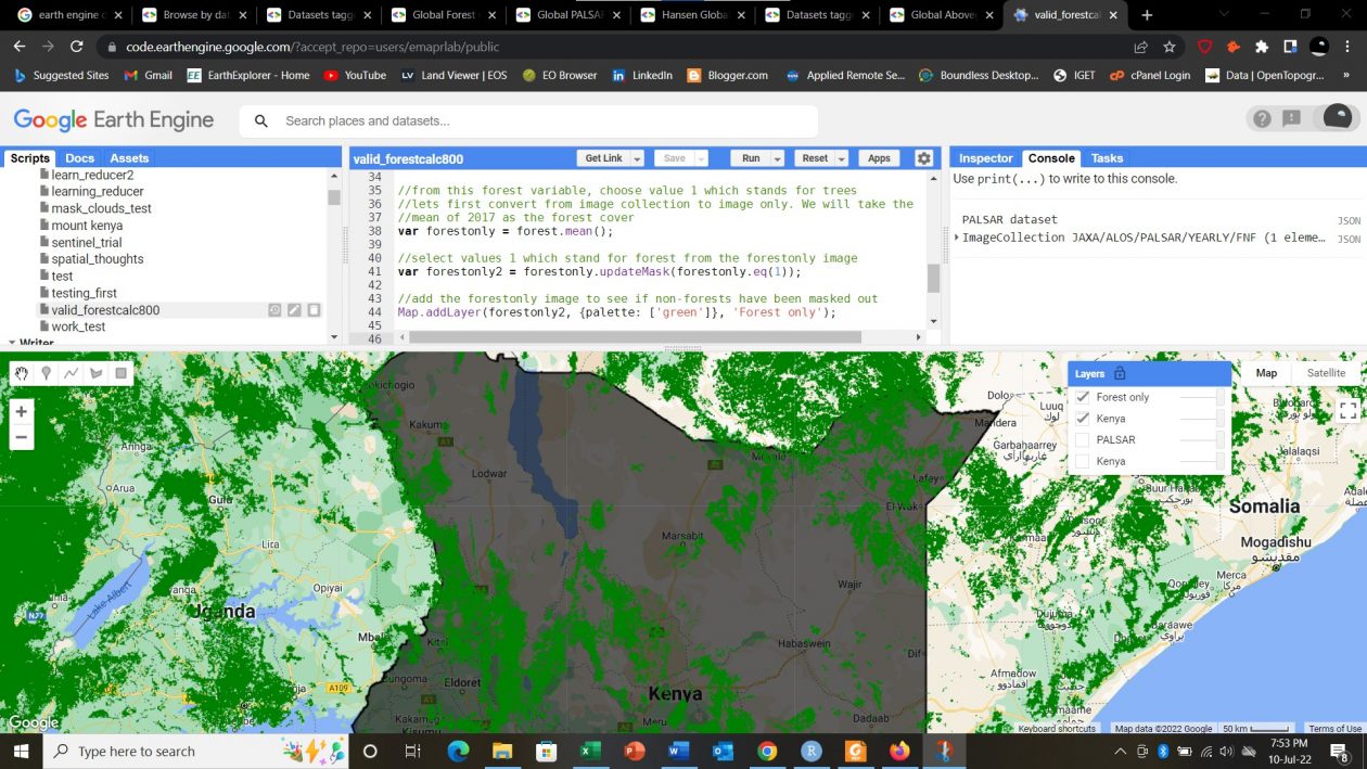
Clip forest coverage to Kenya only
Like carving out the silhouette from a canvas, we want to extract the forest cover in Kenya only.
//now time to clip to Kenya only
var kenyaForests = forestonly2.clip(Kenya);

//lets see forests in Kenya only
Map.addLayer(kenyaForests, {palette: ['green']}, 'Forests in Kenya');

//so far so good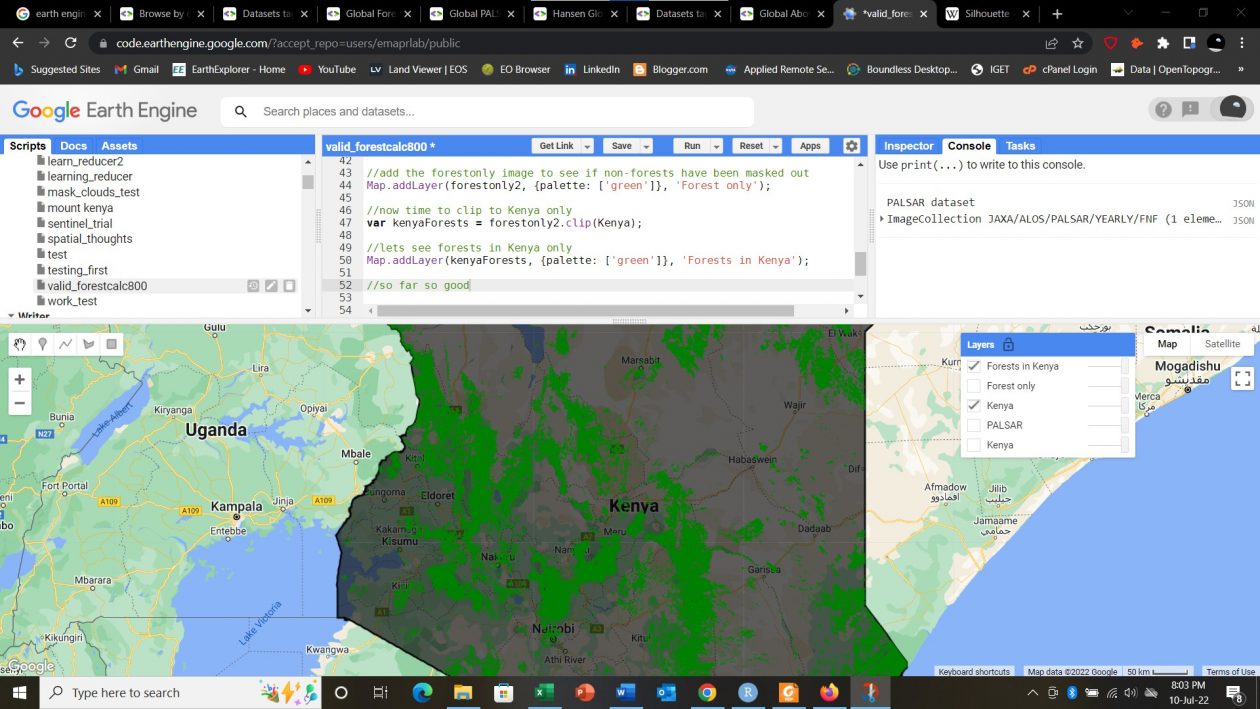
Calculate the area of forest cover in Kenya
Now to the real deal. Time to calculate the area of forest cover in Kenya. For one, we already know the KFS 2021 report put this at 5,226,191.79ha or 5,2261.9179 km2. What will we get?
// lets make these pixels of forests have an attribute of area, to help in
//calculations
print("Forest in Kenya", kenyaForests); //to get a feel of the data

var forestArea = kenyaForests.multiply(ee.Image.pixelArea());

print("Forests with area attribute", forestArea);

//the help says that the ee.Image.pixelArea() shall return a band
//called 'area'. However, our image, does not have this band 'area'.

//so far, so good, maybe
The method ee.Image.pixelArea() mentions that it will return the image output with a band called area but this was not the case.
Print the area statistics for forest cover in Kenya
They say, put your money where your mouth is. We shall say, put a number on what the area is.
Here is the script for printing the area statistics of Kenya’s forest cover in metres. Remember the method ee.Image.pixelArea() assigned the value of every pixel with its corresponding area value in square metres.
//calculate the area of forests in Kenya

var forestedArea = forestArea.reduceRegion({
  reducer: ee.Reducer.sum(),        //research more on reducers
  geometry: Kenya,         //the region to reduce data to or operating area
  scale: 10,           //the scale in meters to work in, went with Sentinel2
  crs: 'epsg:32737',   //used local projection WGS 84 UTM zone 37S
  bestEffort: true,   //used true so that server could determine its own best
  maxPixels: 1e7     //the default of 10000000
});

print("forestedArea", forestedArea);
This was our result:
fnf: 126804959158.53334fnf was the band for forest cover only in the Global PALSAR dataset.
Now, to put the final nail in the coffin.
Get area statistics of forest cover in km2 and ha
To calculate the area statistics in km2 and ha, the below scripts were run.
//get total forested area in sq km
var forestKm = ee.Number(forestedArea.get('fnf')).divide(1e6);
print('Area of forests in sq kilometers: ', forestKm);

//get total forested area in ha
var forestHa = ee.Number(forestedArea.get('fnf')).divide(1e4);  //a ha = 10000sq. metres
print('Area of forests in hectares: ', forestHa);
The results were as follows:
Area of forests in sq kilometers:
126804.95915853334
Area of forests in hectares:
12680495.915853335
Using just the ha statistics, it’s like Kenya has 7 million hectares of forests more than those reported in the KFS 2021 report – 5,226,191.79ha. Using land area, this is like 22% of the country. Lol.
Why the discrepancy? It had something to do with the wrong classification of the Global PALSAR dataset or its 25-m resolution. A more likely explanation is that the Global PALSAR dataset also classified scattered trees and clumped this up with larger forest blocks indiscriminately.
End of Phase 1.
Beginning of Phase 2.
Disaggregating the forest cover area to counties
Below is the code that was used to disaggregate forest area statistics for each county. A new attribute column sum was added to the original forestArea data.
//disaggregated the forestedArea statistics to each county

var countyForests = forestArea.reduceRegions({
  collection: counties,
  reducer: ee.Reducer.sum(),  //calculate the sum area of forestedArea per county
  scale: 10,             //chose a resolution same as that of Sentinel 2
  crs: 'epsg:32737'     //used a local datum of WGS 84 Zone 37S
});

print('Area of forests in counties: ', countyForests);
You will now notice that the output countyForests data has a column sum which is the result of the reducer ee.Reducer.sum(). Once again, research on the term reducer. You will be grateful in that it will reduce some fuzziness on this term. In the case of feature property 0 which stands for Baringo county, the sum attribute, or the forest area cover for this county is 7300173368.107181 square metres.
ADM1_EN: Baringo
...
sum: 7300173368.107181
...
You may have asked why the forestedArea data was not used, since it was the last result just before applying the reducRegions() function. Using this resulted in an error shown below.
Line 98: forestedArea.reduceRegions is not a function
In order to get around this problem, the forestArea data, which came before ee.Image.pixelArea() was applied, was used. It still contains the same data as for forestedArea, except that the pixels have not calculated their area values yet.
Export results to google drive
The GEE has functionalities that enable the user to send data to various cloud storage platforms.
Here is the script to export the area statistics table to your google drive folder. It will be worth the effort to read about the Export.table.toDrive() method of GEE.
Export.table.toDrive({
  collection: countyForests,    //the table with forest area statistics per county
  description: 'county_forestarea_metres', //the title of the table
  folder: 'test',   //the folder the table will be saved into
  fileFormat: 'CSV'
});
Calculations of county forest cover in km2 and ha were done in google sheets and Qgis.
Calculate the percentage of forest cover in each county
Some counties may be large but with small forest coverage. Conversely, some small counties have high forest coverage. To normalize our results, percentages of forest coverage were done for each county.
The methodology was as follows:
- The spatial area of each county in km2 was calculated in Qgis. This attribute was then joined to that of the google sheets (after km2 and ha have been derived).
- The joined table was saved as an excel workbook.
- The percentage calculation of each forest coverage per county was done through the following equation in excel.
(A/B) * 100 where:

A is the forest coverage are for each county in km2 (Area_km)
B is the spatial area for each county in km2 (County_Area_km)
The KFS 2021 report shows the forest cover percentage for all the counties. The top five counties are Nyeri, Lamu, Kilifi, Nyandarua and Bomet.
In our results, however, it is a paradox. The top five counties are Baringo, West Pokot, Elgeyo Marakwet, Nyeri and Murang’a. Where could we have gone wrong?
#show the results of forest cover percentage for each county

#show top six counties with largest forest cover percentage

## # A tibble: 6 x 8
##   ADM0_EN ADM1_EN                  date       sum Area_km Area_ha County_Area_km
##   <chr>   <chr>                   <dbl>     <dbl>   <dbl>   <dbl>          <dbl>
## 1 Kenya   Baringo         1509692400000   7.30e 9   7300.  7.30e5         10889.
## 2 Kenya   West Pokot      1509692400000   6.22e 9   6215.  6.22e5          9306.
## 3 Kenya   Elgeyo-Marakwet 1509692400000   1.92e 9   1920.  1.92e5          3008.
## 4 Kenya   Nyeri           1509692400000   1.92e 9   1920.  1.92e5          3335.
## 5 Kenya   Murang'a        1509692400000   1.36e 9   1365.  1.36e5          2526.
## 6 Kenya   Kitui           1509692400000   1.41e10  14146.  1.41e6         30457.
## # ... with 1 more variable: `Percentage forest Area` <dbl>
All fingers point to the Global PALSAR dataset. By adding the map.addLayer() method to GEE, you will notice that some of the arid counties–which are the notorious top three in our resultant table data–have some of the highest forest coverage per land area.
Nothing could be further from the truth.
//view the forest coverage in counties
Map.addLayer(counties, {}, 'Counties');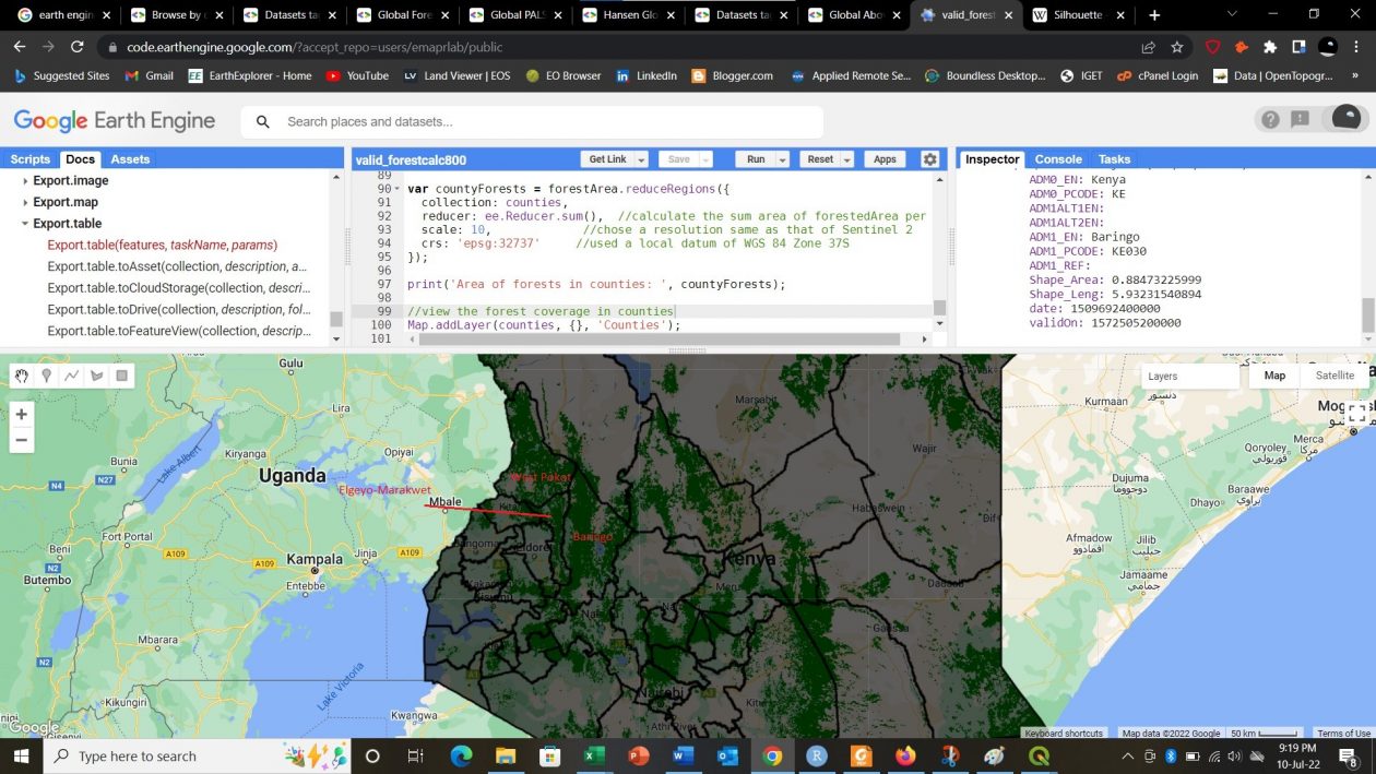
Conclusion
Though with unexpected results, the above was a simple workflow for forest cover assessment in a country using desktop research. Arguably, it has also brought to the fore why higher resolution will always be a call for most studies.
This is because higher resolutions reduce chances of generalization, whereby certain land covers can be classified wrongly, such as the likelihood of woodland or scattered trees still being categorized as forest.
Nevertheless, the use of powerful AI tools such as GEE enable researchers to conduct their own background studies to either corroborate, verify or refute certain studies that may have otherwise been published or publicized. Alternatively, at points where results may fall far short of what is already acknowledged as accurate, other statistical measurements such as standard deviation to identify the margin of error can be used. The results of this work can serve as a point of departure. It was not work in vain.
Forest coverage in counties
##    ADM0_EN         ADM1_EN         date         sum  Area_km    Area_ha
## 1    Kenya         Baringo 1.509692e+12  7300173368  7300.17  730017.34
## 2    Kenya      West Pokot 1.509692e+12  6215088616  6215.09  621508.86
## 3    Kenya Elgeyo-Marakwet 1.509692e+12  1919553427  1919.55  191955.34
## 4    Kenya           Nyeri 1.509692e+12  1919625779  1919.63  191962.58
## 5    Kenya        Murang'a 1.509692e+12  1364808462  1364.81  136480.85
## 6    Kenya           Kitui 1.509692e+12 14146377144 14146.38 1414637.71
## 7    Kenya       Kirinyaga 1.509692e+12   679056736   679.06   67905.67
## 8    Kenya         Kericho 1.509692e+12  1141081192  1141.08  114108.12
## 9    Kenya            Lamu 1.509692e+12  2564613887  2564.61  256461.39
## 10   Kenya          Kiambu 1.509692e+12  1066365916  1066.37  106636.59
## 11   Kenya         Mandera 1.509692e+12 10257178183 10257.18 1025717.82
## 12   Kenya         Samburu 1.509692e+12  8269434150  8269.43  826943.41
## 13   Kenya     Trans Nzoia 1.509692e+12   956571720   956.57   95657.17
## 14   Kenya           Bomet 1.509692e+12   854856391   854.86   85485.64
## 15   Kenya            Meru 1.509692e+12  2398656929  2398.66  239865.69
## 16   Kenya           Nandi 1.509692e+12   947915158   947.92   94791.52
## 17   Kenya            Embu 1.509692e+12   912337543   912.34   91233.75
## 18   Kenya   Tharaka-Nithi 1.509692e+12   830983192   830.98   83098.32
## 19   Kenya           Kisii 1.509692e+12   412830466   412.83   41283.05
## 20   Kenya         Nyamira 1.509692e+12   276010302   276.01   27601.03
## 21   Kenya         Nairobi 1.509692e+12   208895198   208.90   20889.52
## 22   Kenya       Nyandarua 1.509692e+12   957839381   957.84   95783.94
## 23   Kenya          Nakuru 1.509692e+12  2174109541  2174.11  217410.95
## 24   Kenya          Kilifi 1.509692e+12  3365582568  3365.58  336558.26
## 25   Kenya         Mombasa 1.509692e+12    61467500    61.47    6146.75
## 26   Kenya         Garissa 1.509692e+12  9252932604  9252.93  925293.26
## 27   Kenya           Narok 1.509692e+12  3563396689  3563.40  356339.67
## 28   Kenya    Taita Taveta 1.509692e+12  3308754376  3308.75  330875.44
## 29   Kenya         Makueni 1.509692e+12  1331737655  1331.74  133173.77
## 30   Kenya     Uasin Gishu 1.509692e+12   541016675   541.02   54101.67
## 31   Kenya          Isiolo 1.509692e+12  3962383357  3962.38  396238.34
## 32   Kenya      Tana River 1.509692e+12  5843615791  5843.62  584361.58
## 33   Kenya           Wajir 1.509692e+12  7137564402  7137.56  713756.44
## 34   Kenya           Kwale 1.509692e+12   944596929   944.60   94459.69
## 35   Kenya         Turkana 1.509692e+12  7816033471  7816.03  781603.35
## 36   Kenya          Vihiga 1.509692e+12    56760134    56.76    5676.01
## 37   Kenya        Marsabit 1.509692e+12  7679984672  7679.98  767998.47
## 38   Kenya        Kakamega 1.509692e+12   297926598   297.93   29792.66
## 39   Kenya         Bungoma 1.509692e+12   286252975   286.25   28625.30
## 40   Kenya         Kajiado 1.509692e+12  1942974510  1942.97  194297.45
## 41   Kenya        Laikipia 1.509692e+12   808356882   808.36   80835.69
## 42   Kenya        Homa Bay 1.509692e+12   149993542   149.99   14999.35
## 43   Kenya        Machakos 1.509692e+12   174205360   174.21   17420.54
## 44   Kenya          Kisumu 1.509692e+12    72402463    72.40    7240.25
## 45   Kenya           Busia 1.509692e+12    42206501    42.21    4220.65
## 46   Kenya           Siaya 1.509692e+12    38714252    38.71    3871.43
## 47   Kenya          Migori 1.509692e+12    30384458    30.38    3038.45
##    County_Area_km Percentage forest Area
## 1         10889.2             67.0404621
## 2          9305.5             66.7894256
## 3          3008.4             63.8063422
## 4          3334.6             57.5670245
## 5          2525.5             54.0411800
## 6         30456.8             46.4473615
## 7          1475.3             46.0286044
## 8          2513.2             45.4034697
## 9          6047.0             42.4112783
## 10         2543.0             41.9335431
## 11        25979.3             39.4821262
## 12        21015.7             39.3488202
## 13         2484.7             38.4984103
## 14         2438.2             35.0611107
## 15         6992.5             34.3033250
## 16         2835.8             33.4268989
## 17         2823.7             32.3100896
## 18         2581.0             32.1960480
## 19         1313.7             31.4249829
## 20          897.2             30.7634864
## 21          707.5             29.5265018
## 22         3266.7             29.3213335
## 23         7487.1             29.0380788
## 24        12599.3             26.7124364
## 25          233.6             26.3142123
## 26        43596.0             21.2242637
## 27        17912.2             19.8937037
## 28        17131.1             19.3142880
## 29         8174.9             16.2905968
## 30         3396.8             15.9273434
## 31        25399.3             15.6003512
## 32        39192.2             14.9101607
## 33        56668.6             12.5952644
## 34         8266.0             11.4275345
## 35        70131.8             11.1447731
## 36          560.5             10.1266726
## 37        76027.8             10.1015418
## 38         3008.0              9.9045878
## 39         3016.2              9.4904184
## 40        21884.8              8.8781712
## 41         9536.9              8.4761296
## 42         4731.9              3.1697627
## 43         6044.3              2.8822196
## 44         2665.0              2.7166979
## 45         1811.6              2.3299845
## 46         3520.4              1.0995910
## 47         3144.3              0.9661928


Forest cover assessment using GEE