Introduction
Before we get into how to create a web map in R, let’s first know what R is. R is a statistical and computing language first developed in the early 1990s. Ever since then, it has grown in leaps and bounds in terms of development and usage. Apart from statistics, R is also used for cartography and spatial analyses. This is where the RStudio comes in. RStudio is an Integrated Development Environment (IDE) for the R Language, in other words, the GUI for writing R code. You can consider RStudio as the more ‘beautiful’ site for writing the R language. Don’t take my word for it, just judge the book by its cover for yourself by counterchecking the interfaces of R versus RStudio yourself.
Did we mention you can do spatial analyses in R? Not only spatial analyses but also making web maps out of them. Today, we will look at how to create a web map in R and also include a few GIS operations. When we mention R, take it as the R languages appearing in RStudio. Time to spin the decks with our RStudio.
The most famous tool used to create a web map in RStudio is the Leaflet package. The Leaflet package is powered by Javascript and is called into R using the library function. One can also create a web map using the tmap package but that’s a story for another day.
Today, we will create a web map of Kenyan wards showcasing dummy electoral results. A raster file will also be loaded to demonstrate a few functionalities. For the political diehards, the numbers used herein are in no way representative or reflective of the true results to be counted on voting day.
In R, packages are a collection of functions that run certain processes or produce certain outputs. Packages in R are stored in a directory called a library. For those packages not installed in R by default, they are called into the R environment using library(). An example of this will be the packages which we need for spatial operations as shown below.
NB: If installing a package for the first time, use install.packages() and thereafter load it into R with library(package name).
library(sp)
library(sf)
library(rgeos)
library(rgdal)
## Please note that rgdal will be retired by the end of 2023,
## plan transition to sf/stars/terra functions using GDAL and PROJ
## at your earliest convenience.
## rgdal: version: 1.5-28, (SVN revision 1158)
## Geospatial Data Abstraction Library extensions to R successfully loaded
## Loaded GDAL runtime: GDAL 3.2.1, released 2020/12/29
## Path to GDAL shared files: C:/Users/User/Documents/R/win-library/4.1/rgdal/gdal
## GDAL binary built with GEOS: TRUE
## Loaded PROJ runtime: Rel. 7.2.1, January 1st, 2021, [PJ_VERSION: 721]
## Path to PROJ shared files: C:/Users/User/Documents/R/win-library/4.1/rgdal/proj
## PROJ CDN enabled: FALSE
## Linking to sp version:1.4-6
## To mute warnings of possible GDAL/OSR exportToProj4() degradation,
## use options("rgdal_show_exportToProj4_warnings"="none") before loading sp or rgdal.
## Overwritten PROJ_LIB was C:/Users/User/Documents/R/win-library/4.1/rgdal/proj
library(leaflet)
This is just for starters but more packages will be added. In fact, more often than not, you will be using library to add more packages as you progress in handling more sophisticated tasks. There might arise a need where you may have to create one yourself!
Find a description of each of the above packages.
Load the shapefile
Let’s load the shapefile we will use to create a web map. The shapefile is available here. Save and extract it in your directory.
kenya_wards <- readOGR(dsn = "D:/gis-articles-800/leaflet/kenya_wards.shp")
## OGR data source with driver: ESRI Shapefile
## Source: "D:\gis-articles-800\leaflet\kenya_wards.shp", layer: "kenya_wards"
## with 1450 features
## It has 5 fields
## Integer64 fields read as strings:  gid
Leaflet
Earlier in this article, we mentioned that the Leaflet package is used to create a web map. Let’s see how it looks without any data parsed into it.
# make a leaflet widget
leaflet()
A plain grey cold looking map.
Leaflet, according to the help menu, is a function to create a Leaflet map widget. This is what you see above.
Add map tiles
Our map can’t be blank. We will spice things up by adding some base maps. Base maps are added using addTiles(), part of the functions within the leaflet package. addTiles() adds maptiles, which are collections of joined square boxes of the requested image or vector data.
leaflet() %>%
  addTiles() # you can see a global map appears and all seven continents shown twice in one view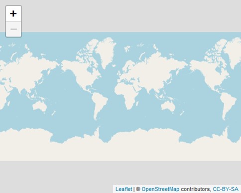
You can see a base map of the globe has been added. However, it has been replicated thrice! This is because no spatial object, which can refer to a place on the earth’s surface, has been added.
Add polygons
Let’s add a spatial object, our kenya_wards shapefile.
# add kenya wards map to leaflet
leaflet() %>%
  addTiles() %>%
  addPolygons(data = kenya_wards) # you can see that the kenya wards shapefile was added to leaflet
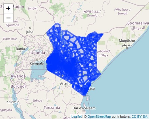
You may have noticed that it took some time for it to load. That is not good news for something that will go online at some point. Just how long was the delay?
# check loading time
start_time <- Sys.time()
leaflet() %>%
  addTiles() %>%
  addPolygons(data = kenya_wards)
end_time <- Sys.time()
difference <- end_time - start_time
difference
## Time difference of 29.35892 secs
Twenty seconds? Enough to do a 100m sprint and back. Let’s reduce the size of this shapefile using the rmapshaper package. As a matter of fact, we will reduce it without using library() to call the package into R. How? A simple:: does the trick.
# reduce size of shapefile
kenya_wards2 <- rmapshaper::ms_simplify(input = kenya_wards, keep = 0.03, keep_shapes = T)
## Registered S3 method overwritten by 'geojsonlint':
##   method         from
##   print.location dplyr
Let’s reload the leaflet map with the simplified kenya_wards2 spatial object. We will also check the time it takes to load each and know who is faster now.
# compare with kenya_wards2 shapefile
start_time <- Sys.time()
leaflet() %>%
  addTiles() %>%
  addPolygons(data = kenya_wards2)
end_time <- Sys.time()
difference <- end_time - start_time
difference
## Time difference of 5.062881 secsFive seconds?! The loading time just got reduced by more than half.
# draw leaflet map with kenya_wards2
leaflet() %>%
  addTiles() %>%
  addPolygons(data = kenya_wards2)
Join spatial object with data frame
To view the attributes for a shapefile, the @data suffix is added after the shapefile name. This is unlike working with tables where, simply calling their name, displays R displays as many of the table’s attributes as it can handle.
head(kenya_wards2@data)  # show first six attribute rows
##    gid pop2009 county         subcounty                   ward
## 1  241   17431 ISIOLO Isiolo Sub County                 WABERA
## 2 1455   18755 Migori  Rongo Sub County   North Kamagambo Ward
## 3 1456   27756 Migori  Rongo Sub County Central Kamagambo Ward
## 4 1457   27179 Migori  Rongo Sub County   South Kamagambo Ward
## 5 1458   22874 Migori Awendo Sub County       North Sakwa Ward
## 6 1459   36200 Migori Awendo Sub County       South Sakwa Ward
Alright. We promised our web map would show both administrative and electoral result attributes. Looking at it, only administrative attributes can be seen. Luckily, We have a curated table showing the dummy electoral results.
# load the table with voter data
ward_data <- read.csv("D:/gis-articles-800/leaflet/wards_full.csv", header = T)
head(ward_data)
##   X  gid pop2009 county         subcounty                   ward         uid
## 1 1  241   17431 ISIOLO Isiolo Sub County                 WABERA rIdiIpv9fBt
## 2 2 1455   18755 Migori  Rongo Sub County   North Kamagambo Ward QC41mItjIzF
## 3 3 1456   27756 Migori  Rongo Sub County Central Kamagambo Ward M8rGveWTIMm
## 4 4 1457   27179 Migori  Rongo Sub County   South Kamagambo Ward DABObbHgPMX
## 5 5 1458   22874 Migori Awendo Sub County       North Sakwa Ward EmSsP2C6A3h
## 6 6 1459   36200 Migori Awendo Sub County       South Sakwa Ward OpbsijPbYuv
##         scuid        cuid voters david_waih george_waj raila_odin reuben_kig
## 1 I2LYLqKU6AW bzOfj0iwfDH   1779         39         66         52         79
## 2 fT37q3rXQ35 fVra3Pwta0Q   1682         69         52         17         94
## 3 fT37q3rXQ35 fVra3Pwta0Q   1232         18         94         11         30
## 4 fT37q3rXQ35 fVra3Pwta0Q   1991         21         25         25         59
## 5 ka9Uv3Ckcbd fVra3Pwta0Q   1065         33         33         67         29
## 6 ka9Uv3Ckcbd fVra3Pwta0Q   1986         74         39         84         93
##   william_ru
## 1         56
## 2         95
## 3         86
## 4         97
## 5         97
## 6         60
Question is, just how do we take the columns from voters to william_ru and join them to our spatial kenya_wards2? In QGIS, we could do it using the joins tool. R also has its own tricks up its sleeve for the same purpose.
Actually, the original kenya_wards shapefile contains all the electoral data when viewed in QGIS. It was created in Qgis using the joins tool alluded to earlier. For some reason, however, these electoral data columns are not visible when loaded in R. Nevertheless, we will take the bull by its horns and merge these electoral attributes with our shapefile so that eventually our shapefile is in top-notch shape.
The sp package has the merge() function which is used to merge a spatial object with a data frame –which in our case is the table above.
kenya_wards3 <- merge(x = kenya_wards2,
                      y = ward_data, by.x = "gid",
                      by.y = "gid", # show which column to join by
                      suffixes = c(".x", ".y")) # add suffixes to differentiate by source
head(kenya_wards3@data)
##      gid pop2009.x county.x       subcounty.x                 ward.x X
## 962  241     17431   ISIOLO Isiolo Sub County                 WABERA 1
## 47  1455     18755   Migori  Rongo Sub County   North Kamagambo Ward 2
## 48  1456     27756   Migori  Rongo Sub County Central Kamagambo Ward 3
## 49  1457     27179   Migori  Rongo Sub County   South Kamagambo Ward 4
## 50  1458     22874   Migori Awendo Sub County       North Sakwa Ward 5
## 51  1459     36200   Migori Awendo Sub County       South Sakwa Ward 6
##     pop2009.y county.y       subcounty.y                 ward.y         uid
## 962     17431   ISIOLO Isiolo Sub County                 WABERA rIdiIpv9fBt
## 47      18755   Migori  Rongo Sub County   North Kamagambo Ward QC41mItjIzF
## 48      27756   Migori  Rongo Sub County Central Kamagambo Ward M8rGveWTIMm
## 49      27179   Migori  Rongo Sub County   South Kamagambo Ward DABObbHgPMX
## 50      22874   Migori Awendo Sub County       North Sakwa Ward EmSsP2C6A3h
## 51      36200   Migori Awendo Sub County       South Sakwa Ward OpbsijPbYuv
##           scuid        cuid voters david_waih george_waj raila_odin reuben_kig
## 962 I2LYLqKU6AW bzOfj0iwfDH   1779         39         66         52         79
## 47  fT37q3rXQ35 fVra3Pwta0Q   1682         69         52         17         94
## 48  fT37q3rXQ35 fVra3Pwta0Q   1232         18         94         11         30
## 49  fT37q3rXQ35 fVra3Pwta0Q   1991         21         25         25         59
## 50  ka9Uv3Ckcbd fVra3Pwta0Q   1065         33         33         67         29
## 51  ka9Uv3Ckcbd fVra3Pwta0Q   1986         74         39         84         93
##     william_ru
## 962         56
## 47          95
## 48          86
## 49          97
## 50          97
## 51          60
You will notice that there are several duplicate columns. We will remove those that we don’t need. These will be the columns denoted with the suffix .y since our shapefile already had them before the merge operation. They are denoted by the suffix .y in our table. We will remove them and remain with the voter data.
kenya_wards4 <- kenya_wards3[ , -c(7:13)] # remove duplicate columns
head(kenya_wards4@data)
##      gid pop2009.x county.x       subcounty.x                 ward.x X voters
## 962  241     17431   ISIOLO Isiolo Sub County                 WABERA 1   1779
## 47  1455     18755   Migori  Rongo Sub County   North Kamagambo Ward 2   1682
## 48  1456     27756   Migori  Rongo Sub County Central Kamagambo Ward 3   1232
## 49  1457     27179   Migori  Rongo Sub County   South Kamagambo Ward 4   1991
## 50  1458     22874   Migori Awendo Sub County       North Sakwa Ward 5   1065
## 51  1459     36200   Migori Awendo Sub County       South Sakwa Ward 6   1986
##     david_waih george_waj raila_odin reuben_kig william_ru
## 962         39         66         52         79         56
## 47          69         52         17         94         95
## 48          18         94         11         30         86
## 49          21         25         25         59         97
## 50          33         33         67         29         97
## 51          74         39         84         93         60
Now we have our electoral data: the voters and results for each of our named aspirants.
Make the web map interactive
Now, to what we have been waiting for. Let’s load these improved kenya_wards2 data to our leaflet map. In addition, we will make the wards clickable. That is, some data will show up on the screen when a particular ward is clicked by the user. The popup argument within the addPolygons() will enable this.
# make the polygons clickable and showing some data of each ward
leaflet() %>%
  addTiles() %>%
  addPolygons(
    data = kenya_wards4,
    popup = paste0("County: ", kenya_wards4@data$county, "<br>",
                   "Ward: ", kenya_wards4@data$ward, "<br>",
                   "Voters: ", kenya_wards4@data$voters, "<br>",
                   "David Waihiga: ", kenya_wards4@data$david_waih, "<br>",
                   "George Wajackoyah: ", kenya_wards4@data$george_waj, "<br>",
                   "Raila Odinga: ", kenya_wards4@data$raila_odin, "<br>",
                   "Reuben Kigame: ", kenya_wards4@data$reuben_kig, "<br>",
                   "William Ruto: ", kenya_wards4@data$william_ru
                   )
    )

# upon clicking you see ward electoral data
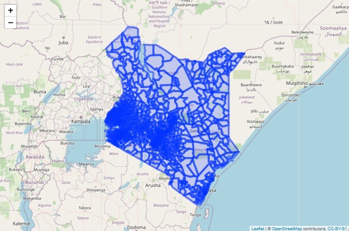
Click on any ward and you will see a popup showing some information about that ward–political (County name and ward name) and electoral (voters, David Waihiga, George Wajackoyah etc).
Furthermore, we can also change the aesthetics. We want to colour-code the wards according to the counties they fall under. This will make it easy to distinguish one county from another, thus also easing the navigation experience. Sounds easy, but it is not. To create the different colour codes, we have to create a colour function using colorFactor(). Once the function is created, it can be parsed to Leaflet for display.
# create a color function for coloring map
color_wards <- colorFactor(palette = topo.colors(47), domain = kenya_wards4@data$county.x)
# create a colored map with wards categorized to their counties by color
leaflet() %>%
  addTiles() %>%
  addPolygons(
    data = kenya_wards4,
    color = ~color_wards(kenya_wards4@data$county.x), # added the color component
    opacity = 0.3, weight = 2,  # to make the colors less opaque and not shouting
    popup = paste0("County: ", kenya_wards4@data$county, "<br>",
                   "Ward: ", kenya_wards4@data$ward, "<br>",
                   "Voters: ", kenya_wards4@data$voters, "<br>",
                   "David Waihiga: ", kenya_wards4@data$david_waih, "<br>",
                   "George Wajackoyah: ", kenya_wards4@data$george_waj, "<br>",
                   "Raila Odinga: ", kenya_wards4@data$raila_odin, "<br>",
                   "Reuben Kigame: ", kenya_wards4@data$reuben_kig, "<br>",
                   "William Ruto: ", kenya_wards4@data$william_ru
                   )
    )
How about making the wards highlight upon mouse hover? This can be done using the highlightOptions() function. As you can see, most of the function names under the leaflet package also hint at their purpose(s).
leaflet() %>%
  addTiles() %>%
  addPolygons(
    data = kenya_wards4,
    color = ~color_wards(kenya_wards4@data$county.x), # added the color component
    opacity = 0.3, weight = 2,  # to make the colors less opaque and not shouting
    popup = paste0("County: ", kenya_wards4@data$county, "<br>",
                   "Ward: ", kenya_wards4@data$ward, "<br>",
                   "Voters: ", kenya_wards4@data$voters, "<br>",
                   "David Waihiga: ", kenya_wards4@data$david_waih, "<br>",
                   "George Wajackoyah: ", kenya_wards4@data$george_waj, "<br>",
                   "Raila Odinga: ", kenya_wards4@data$raila_odin, "<br>",
                   "Reuben Kigame: ", kenya_wards4@data$reuben_kig, "<br>",
                   "William Ruto: ", kenya_wards4@data$william_ru
                   ),
    highlightOptions = highlightOptions(
      stroke = T,
      color = "white",
      weight = 5,
      opacity = 0.5,
      bringToFront = T
      ), # made the wards highlightable on hover
    )
The addMarker() would have been a nice complimenter to the highlightsOptions function in that it would show a label–such as a ward’s name–upon mouse hover. However, the addMarker() function needs longitude and latitude information, not included in our data and thus we prefer to explore it on another day.
Add base maps
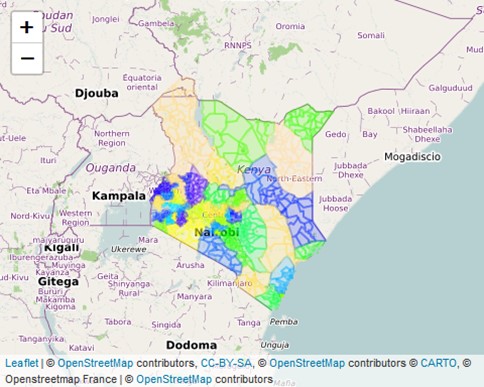
Currently, our map contains only one base map layer, the default Open StreetMap (OSM) base map that comes with the leaflet package. However, we can add more base maps using the addProviderTiles() function.
#
leaflet() %>%
  addTiles(
    group = "OSM"
    ) %>% # the default web map layer is OSM, so we put into group name 'OSM'.
  addProviderTiles(
    providers$CartoDB.Positron, group = "Carto"
    ) %>% # added an extra webmap layer and called group - CartoDB
  addProviderTiles(
    providers$OpenStreetMap.France,
    group = "OSM France"
    ) %>% #added an extra webmap layer called group - OSM France
  addPolygons(
    data = kenya_wards4,
    color = ~color_wards(kenya_wards4@data$county.x), # added the color component
    opacity = 0.3, weight = 2,  # to make the colors less opaque and not shouting
    popup = paste0("County: ", kenya_wards4@data$county, "<br>",
                   "Ward: ", kenya_wards4@data$ward, "<br>",
                   "Voters: ", kenya_wards4@data$voters, "<br>",
                   "David Waihiga: ", kenya_wards4@data$david_waih, "<br>",
                   "George Wajackoyah: ", kenya_wards4@data$george_waj, "<br>",
                   "Raila Odinga: ", kenya_wards4@data$raila_odin, "<br>",
                   "Reuben Kigame: ", kenya_wards4@data$reuben_kig, "<br>",
                   "William Ruto: ", kenya_wards4@data$william_ru),
    highlightOptions = highlightOptions(
      stroke = T,
      color = "white",
      weight = 5,
      opacity = 0.5,
      bringToFront = T
      ), # made the wards highlightable on hover
) 
Add layers control
There is one problem though. We can only see one base map layer. Actually, the base map for ‘OpenStreetMap.France’. For the other two, the user is at a loss for where to retrieve them, and that will be a bad client experience. This problem is solved by the group argument included in our script below. The group argument does what it says – group our layers to a particular unit named by the user.
This still doesn’t answer our question of being able to retrieve any of our other two base maps. For this, we will add a control widget that allows toggling one layer on or off. The addLayersControl() function comes into force.
# we need to add a toggle on or off widget to choose which map layers we want to be visible

leaflet() %>%
  addTiles(
    group = "OSM"
    ) %>% # the default web map layer is OSM, so we put into group name 'OSM'.
  addProviderTiles(
    providers$CartoDB.Positron,
    group = "Carto"
    ) %>% # added an extra webmap layer and called group - CartoDB
  addProviderTiles(
    providers$OpenStreetMap.France,
    group = "OSM France"
    ) %>% #added an extra webmap layer called group - OSM France
  addPolygons(
    data = kenya_wards4,
    color = ~color_wards(kenya_wards4@data$county.x), # added the color component
    opacity = 0.3,
    weight = 2,  # to make the colors less opaque and not shouting
    popup = paste0(
      "County: ", kenya_wards4@data$county, "<br>",
      "Ward: ", kenya_wards4@data$ward, "<br>",
      "Voters: ", kenya_wards4@data$voters, "<br>",
      "David Waihiga: ", kenya_wards4@data$david_waih, "<br>",
      "George Wajackoyah: ", kenya_wards4@data$george_waj, "<br>",
      "Raila Odinga: ", kenya_wards4@data$raila_odin, "<br>",
      "Reuben Kigame: ", kenya_wards4@data$reuben_kig, "<br>",
      "William Ruto: ", kenya_wards4@data$william_ru
      ),
    highlightOptions = highlightOptions(
      stroke = T,
      color = "white",
      weight = 5,
      opacity = 0.5,
      bringToFront = T
      ), # made the wards highlightable on hover
    group = "administrative"
    ) %>% # put our polygons into the 'administrative' group
  addLayersControl(
    baseGroups = c(
      "OSM", "Carto", "OSM France"
      ), # group names of our OSM layers
    overlayGroups = c(
      "administrative"
      )
    ) # group name for our polygons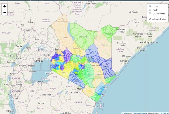
Add raster data
So far, we have worked with vector data. How about raster data? To work with raster data in R, one has to use the raster and terra packages.
# load the terra and raster packages
library(terra)
## terra 1.5.21
##
## Attaching package: 'terra'
## The following object is masked from 'package:rgdal':
##
##     project
library(raster)
## Warning: package 'raster' was built under R version 4.1.3
We will use the rast function from the terra package to load the raster data into R Studio.
# load raster into R
landcover <- rast(x = "D:/gis-articles-800/leaflet/kenya_landcover_2017/kenya_landcover_2017.tif")
landcover  #check attributes
## class       : SpatRaster
## dimensions  : 34481, 29679, 1  (nrow, ncol, nlyr)
## resolution  : 0.0002694946, 0.0002694946  (x, y)
## extent      : 33.907, 41.90533, -4.669802, 4.622641  (xmin, xmax, ymin, ymax)
## coord. ref. : lon/lat WGS 84 (EPSG:4326)
## source      : kenya_landcover_2017.tif
## color table : 1
## categories  : Red, Green, Blue, Type
## name        : Red
## min value   :   0
## max value   : 255
However, this raster is too large to work with. It will not only take much time to load into Leaflet, but it will cause errors to appear when forced into this lightweight (yet powerful) R package tool. Believe me, when it comes to working with Leaflet and any other web-based application, size matters. In R, the aggregate function reduces the resolution of a raster and subsequently also reduces the size of the file.
#reduce size of this raster
landcover2 <- terra::aggregate(landcover, fact=100, fun = "mean", overwrite = T)
landcover2
## class       : SpatRaster
## dimensions  : 345, 297, 1  (nrow, ncol, nlyr)
## resolution  : 0.02694946, 0.02694946  (x, y)
## extent      : 33.907, 41.91099, -4.674923, 4.622641  (xmin, xmax, ymin, ymax)
## coord. ref. : lon/lat WGS 84 (EPSG:4326)
## source      : memory
## name        : Red
## min value   :   1
## max value   :   6
In RStudio, our landcover2 is registered as a SpatRaster file. This will cause issues upon loading to leaflet() which strictly requires a RasterLayer object. We are not geniuses to know this beforehand, rather, we discovered this by experience when we were parsing the landcover2 to leaflet and R splashed the following error into our faces as if to say: “No, thank you”.
Error in addRasterImage(., landcover2, colors = "Spectral", opacity = 0.8,  :
  inherits(x, "RasterLayer") is not TRUE
The raster() function will convert our landcover2 into a RasterLayer object.
# convert to raster layer object
landcover3 <- raster::raster(landcover2)
Time to add the raster to our leaflet map.
###
leaflet() %>%
  addTiles(
    group = "OSM"
    ) %>% # the default web map layer is OSM, so we put into group name 'OSM'.
  addProviderTiles(
    providers$CartoDB.Positron,
    group = "Carto"
    ) %>% # added an extra webmap layer and called group - CartoDB
  addProviderTiles(
    providers$OpenStreetMap.France,
    group = "OSM France"
    ) %>% #added an extra webmap layer called group - OSM France
  addPolygons(
    data = kenya_wards4,
    color = ~color_wards(kenya_wards4@data$county.x), # added the color component
    opacity = 0.3,
    weight = 2,  # to make the colors less opaque and not shouting
    popup = paste0(
      "County: ", kenya_wards4@data$county, "<br>",
      "Ward: ", kenya_wards4@data$ward, "<br>",
      "Voters: ", kenya_wards4@data$voters, "<br>",
      "David Waihiga: ", kenya_wards4@data$david_waih, "<br>",
      "George Wajackoyah: ", kenya_wards4@data$george_waj, "<br>",
      "Raila Odinga: ", kenya_wards4@data$raila_odin, "<br>",
      "Reuben Kigame: ", kenya_wards4@data$reuben_kig, "<br>",
      "William Ruto: ", kenya_wards4@data$william_ru
      ),
    highlightOptions = highlightOptions(
      stroke = T,
      color = "white",
      weight = 5,
      opacity = 0.5,
      bringToFront = T
      ), # make wards highlightable
    group = "administrative",  # put polygons into a group called 'administrative'
  ) %>%
  addRasterImage(
    landcover3,
    colors = rainbow(6),
    opacity = .8,
    group = "landcover",
    layerId = "land_cover"
    ) %>%
  addLayersControl(
    baseGroups = c(
      "OSM", "Carto", "OSM France"
      ), # the group names of our OSM layers
    overlayGroups = c(
      "administrative"
      )
    ) # group name for our polygons
## Warning in showSRID(uprojargs, format = "PROJ", multiline = "NO", prefer_proj =
## prefer_proj): Discarded ellps WGS 84 in Proj4 definition: +proj=merc +a=6378137
## +b=6378137 +lat_ts=0 +lon_0=0 +x_0=0 +y_0=0 +k=1 +units=m +nadgrids=@null
## +wktext +no_defs +type=crs
## Warning in showSRID(uprojargs, format = "PROJ", multiline = "NO", prefer_proj =
## prefer_proj): Discarded datum World Geodetic System 1984 in Proj4 definition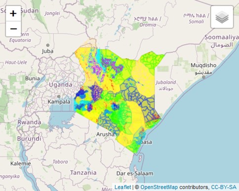
Note that we have updated the addRasterImage() with the group and layerId arguments. addRasterImage adds a raster to Leaflet. As you saw earlier, the group enables the control widget to know which layer to toggle on/off. The layerId is for parsing into an opacity slider, which we shall work with shortly.
Our raster contains colour codes that signify the land cover of that particular region. The colour codes are labelled using numbers. Even though we would prefer real-world names like forestcover, water et cetera to numerical codes, we will use them as they are for today. Numbers don’t lie anyway!
Add legend
A legend is a map element that elaborates on some map features. In Leaflet, it is added using the addLegend() function.
leaflet() %>%
  addTiles(
    group = "OSM"
    ) %>% # the default web map layer is OSM, so we put into group name 'OSM'.
  addProviderTiles(
    providers$CartoDB.Positron,
    group = "Carto"
    ) %>% # added an extra webmap layer and called group - CartoDB
  addProviderTiles(
    providers$OpenStreetMap.France,
    group = "OSM France"
    ) %>% #added an extra webmap layer called group - OSM France
  addPolygons(
    data = kenya_wards4,
    color = ~color_wards(kenya_wards4@data$county.x), # added the color component
    opacity = 0.3,
    weight = 2,  # to make the colors less opaque and not shouting
    popup = paste0(
      "County: ", kenya_wards4@data$county, "<br>",
      "Ward: ", kenya_wards4@data$ward, "<br>",
      "Voters: ", kenya_wards4@data$voters, "<br>",
      "David Waihiga: ", kenya_wards4@data$david_waih, "<br>",
      "George Wajackoyah: ", kenya_wards4@data$george_waj, "<br>",
      "Raila Odinga: ", kenya_wards4@data$raila_odin, "<br>",
      "Reuben Kigame: ", kenya_wards4@data$reuben_kig, "<br>",
      "William Ruto: ", kenya_wards4@data$william_ru
      ),
    highlightOptions = highlightOptions(
      stroke = T,
      color = "white",
      weight = 5,
      opacity = 0.5,
      bringToFront = T
      ), # make wards highlightable
    group = "administrative",  # put polygons into a group called 'administrative'
  ) %>%
  addRasterImage(
    landcover3,
    colors = rainbow(6),
    opacity = .8,
    group = "landcover",
    layerId = "land_cover"
    ) %>%   # add raster layer
  addLegend(
    data = landcover3,
    position = "bottomleft",
    colors = rainbow(6),
    opacity = 0.5,
    labels = c(
      '1', '2', '3', '4', '5', '6'
      ),
    title = "Land classes"
    ) %>% # add legend
  addLayersControl(
    baseGroups = c(
      "OSM", "Carto", "OSM France"
      ), #group names of our OSM layers
    overlayGroups = c(
      "administrative"
      )
    )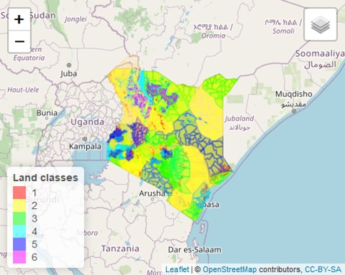
In the addLegend function, the number of label names should match that of the colour codes otherwise, R will throw an error to your face!
Add an opacity slider
Despite the excitement of dealing with a raster in a web map, our new kid on the block conceals all the underlying layers. One way to solve this is parsing the raster to the addLayerControl widget from where it can be toggled on/off like our OSM layers. A second and preferable option is to create an opacity slider whereby the transparency or opaqueness of the raster will be controlled. The opacity slider is not part of the leaflet package and thus has to be installed separately.
We shall proceed with this second option as it makes our web map more versatile.
# load the opacity slider package
library(leaflet.opacity)
## Warning: package 'leaflet.opacity' was built under R version 4.1.3
Let’s throw the opacity slider into our leaflet map script. Remember the layerId we specified for our raster? It is now put into action.
###
leaflet() %>%
  addTiles(
    group = "OSM"
    ) %>% # the default web map layer is OSM, so we put into group name 'OSM'.
  addProviderTiles(
    providers$CartoDB.Positron,
    group = "Carto"
    ) %>% # added an extra webmap layer and called group - CartoDB
  addProviderTiles(
    providers$OpenStreetMap.France,
    group = "OSM France"
    ) %>% #added an extra webmap layer called group - OSM France
  addPolygons(
    data = kenya_wards4,
    color = ~color_wards(kenya_wards4@data$county.x), # added the color component
    opacity = 0.3,
    weight = 2,  # to make the colors less opaque and not shouting
    popup = paste0(
      "County: ", kenya_wards4@data$county, "<br>",
      "Ward: ", kenya_wards4@data$ward, "<br>",
      "Voters: ", kenya_wards4@data$voters, "<br>",
      "David Waihiga: ", kenya_wards4@data$david_waih, "<br>",
      "George Wajackoyah: ", kenya_wards4@data$george_waj, "<br>",
      "Raila Odinga: ", kenya_wards4@data$raila_odin, "<br>",
      "Reuben Kigame: ", kenya_wards4@data$reuben_kig, "<br>",
      "William Ruto: ", kenya_wards4@data$william_ru
      ),
    highlightOptions = highlightOptions(
      stroke = T,
      color = "white",
      weight = 5,
      opacity = 0.5,
      bringToFront = T
      ), # make wards highlightable
    group = "administrative",  # put polygons into a group called 'administrative'
  ) %>%
  addRasterImage(
    landcover3,
    colors = rainbow(6),
    opacity = .8,
    group = "landcover",
    layerId = "land_cover"
    ) %>%   # add raster layer
  addLegend(
    data = landcover3,
    position = "bottomleft",
    colors = rainbow(6),
    opacity = 0.5,
    labels = c(
      '1', '2', '3', '4', '5', '6'
      ),
    title = "Land classes"
    ) %>% # add legend
  addLayersControl(
    baseGroups = c(
      "OSM", "Carto", "OSM France"
      ), # group names of our OSM layers
    overlayGroups = c(
      "administrative"
      )
    ) %>% # group name for our polygons
  addOpacitySlider(
    layerId = "land_cover"
    )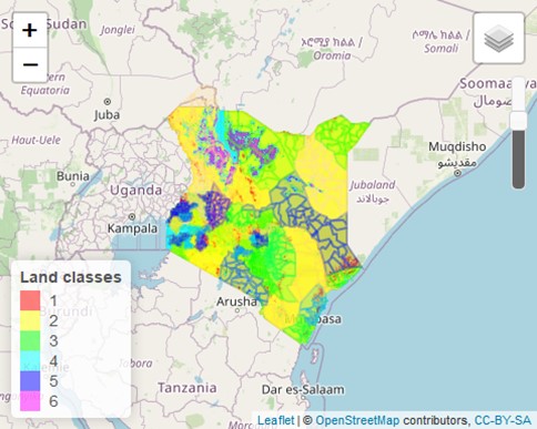
Get adventurous and play around with the opacity slider.
Parse the web map to an object name
Finally, as the icing on the cake, or to cap this long exploration in Leaflet, let us give an object name to our leaflet map script.
leaflet_wards <- leaflet() %>%
  addTiles(
    group = "OSM"
    ) %>% # the default web map layer is OSM, so we put into group name 'OSM'.
  addProviderTiles(
    providers$CartoDB.Positron,
    group = "Carto"
    ) %>% # added an extra webmap layer and called group - CartoDB
  addProviderTiles(
    providers$OpenStreetMap.France,
    group = "OSM France"
    ) %>% #added an extra webmap layer called group - OSM France
  addPolygons(
    data = kenya_wards4,
    color = ~color_wards(kenya_wards4@data$county.x), # added the color component
    opacity = 0.3,
    weight = 2,  # to make the colors less opaque and not shouting
    popup = paste0(
      "County: ", kenya_wards4@data$county, "<br>",
      "Ward: ", kenya_wards4@data$ward, "<br>",
      "Voters: ", kenya_wards4@data$voters, "<br>",
      "David Waihiga: ", kenya_wards4@data$david_waih, "<br>",
      "George Wajackoyah: ", kenya_wards4@data$george_waj, "<br>",
      "Raila Odinga: ", kenya_wards4@data$raila_odin, "<br>",
      "Reuben Kigame: ", kenya_wards4@data$reuben_kig, "<br>",
      "William Ruto: ", kenya_wards4@data$william_ru
      ),
    highlightOptions = highlightOptions(
      stroke = T,
      color = "white",
      weight = 5,
      opacity = 0.5,
      bringToFront = T
      ), # made the wards highlightable on hover
    group = "administrative",  # put polygons into a group called 'administrative'
  ) %>%
  addRasterImage(
    landcover3,
    colors = rainbow(6),
    opacity = .8,
    group = "landcover",
    layerId = "land_cover"
    ) %>%   # add raster layer
  addLegend(
    data = landcover3,
    position = "bottomleft",
    colors = rainbow(6),
    opacity = 0.5,
    labels = c(
      '1', '2', '3', '4', '5', '6'
      ),
    title = "Land classes"
    ) %>% # add legend
  addLayersControl(
    baseGroups = c(
      "OSM", "Carto", "OSM France"
      ), # group names of our OSM layers
    overlayGroups = c(
      "administrative", "landcover"
      )
    ) %>%# group name for our polygons + landcover raster
  addOpacitySlider(
    layerId = "land_cover"
    )

leaflet_wards # all our leaflet map functionalities are encompassed in this name
Like a small bomb that releases its contents to a wide area, so does our object name leaflet_wards work like so. Imagine all those scripts and functions we added are encapsulated in that one name! It’s for a good reason though. When you want to parse this leaflet map to an app, say like in shiny this one name does all the magic needed for the map to appear in your app.
Wrap Up
Leaflet is an extremely useful tool used to create a web map in R, and so far it seems unrivalled. In addition, Leaflet is compatible with other R packages, such as the shiny package for creating apps. Furthermore, Leaflet eliminates the need for the user to learn Javascript since the package does all the interpretation for the user. Javascript is a programming language used in most web-based applications. Were it not for Leaflet, we would have had to crack Javascript to do the above exercise. With a cup of coffee of course.
Cheers, Happy hacking!





Hello, this is so informative.
Can I get access to the landcover raster data that you used. It will be of great help