One of the easiest methods of agricultural remote sensing is the use of the Normalized Difference Moisture Index (NDMI). If you are a good student of GIS and RS, by now you are familiar with NDVI, NDWI, and EVI. NDMI is one of the simplest indices. But let’s not jump before the gun. For starters, what is NDMI?
Kakhovka, Ukraine.
This is one of the hotly fought-over regions between Ukraine and Russia. Currently, it is under the control of Russian forces. Internationally speaking, it belongs to Ukraine. There are plenty of interesting facts about Kakhovka. For one, it is home to the largest irrigation system in Europe. As of 2015, a total of 220, 000 ha was under irrigation. However, it pales in comparison to the Galana Kulalu irrigation project where more than 400, 000 ha are under irrigation. Secondly, its water is fed by the Kakhovka reservoir, built in 1956 and also part of the canal that enables ships to travel from the port to the upper reaches of the Dnieper River.
Because it is the largest irrigation system in Europe, its centre pivot systems and block farms are very distinct from above, thus making it a good candidate for agricultural remote sensing studies. Despite it being the goliath of irrigation systems and wheat production areas in Europe, it has hardly been a subject of remote sensing analyses, if any. Perhaps it’s due to a lack of awareness about it. As a matter of fact, no study has been done to assess the impact of the Russian invasion on the agricultural yields of the Kahkova irrigation system. This is regardless of satellites offering a safe opportunity to venture into these areas without risking a life.
Normalized Difference Moisture Index is a vegetation index that describes the plant’s water stress level. It should not be confused with NDVI which assesses leafy biomass health. NDMI is calculated as the ratio between the difference and the sum of the refracted radiations in the near-infrared (NIR) and Short-wave Infrared (SWIR). That is, (NIR-SWIR)/(NIR+SWIR). According to the Sentinel-2 satellite, which is used in this article, NIR and SWIR belong to band 8 and band 11 respectively.
Normalized Difference Moisture Index enables the identification of farm areas with high water level stress and those without. In an NDMI image, areas with water stress will have negative values falling towards the end of the totem pole of -1. Conversely, areas with abundant water, high vegetation vigour or waterlogged will have sky-high values leaning to +1.
Below is a table showing the range of NDMI values and what they represent.
## # A tibble: 10 x 2
##    `NDMI Values` Interpretation
##    <chr>         <chr>
##  1 1 – -0.8      Bare soil
##  2 -0.8 – -0.6   Almost absent canopy cover,
##  3 -0.6 – -0.4   Very low canopy cover
##  4 -0.4 – -0.2   Low canopy cover, dry or very low canopy cover, wet,
##  5 -0.2 – 0      Mid-low canopy cover, high water stress or low canopy cover, l~
##  6 0 – 0.2       Average canopy cover, high water stress or mid-low canopy cove~
##  7 0.2 – 0.4     Mid-high canopy cover, high water stress or average canopy cov~
##  8 0.4 – 0.6     High canopy cover, no water stress,
##  9 0.6 – 0.8     Very high canopy cover, no water stress,
## 10 0.8 – 1       Total canopy cover, no water stress/waterlogging
Armed with this knowledge, let’s calculate the Normalized Difference Moisture Index value over the Kakhovka irrigation system. Google Earth Engine has an equally fascinating twin brother called Google Earth Engine Pro. Unlike its counterpart, Google Earth Engine Pro prides itself in image visualizations such as 2D and 3D views, time-series lapses and even the display of auxiliary data. Together, they work like two complementary personalities. Google Earth Pro was used to get the coordinates of the Kakhovka Irrigation System. These coordinates were placed into GEE from where we zoomed to our Area of Interest (Kakhovka).
Map.setCenter( 33.788277, 46.471417, 10);In order to get a specific region of Kakhovka to work with, a shapefile from Humanitarian Data Exchange (HDX) was loaded into QGIS and the administrate region of Kakhovka was singled out.
Because the Kakhovka region is dotted and crisscrossed by industries and roads, there was a need to select a solely agricultural field to avoid the influence of man-made features on Normalized Difference Moisture Index values. Therefore, a small bounding box of roughly 4460 hectares was chiselled out and further extended to cover a reasonably large agricultural area.
This bounding box is shown in the script below.
var kakhovka_admin = ee.FeatureCollection("users/sammigachuhi-test/kakhovska_admin"),
    irrigation =
    /* color: #ffc82d */
    /* shown: false */
    ee.Geometry.Polygon(
        [[[33.6678337360909, 46.69377624788908],
          [33.58680956616902, 46.68247182408976],
          [33.59470598950887, 46.65372909846698],
          [33.60328905835652, 46.62155211195734],
          [33.68843310132527, 46.63322290073514]]]);
Here is the Kakhovka administrative region added to the GEE canvas.
// add shapefile for Kakhosvka administration area extracted from this dataset
// https://data.humdata.org/dataset/cod-ab-ukr?

Map.addLayer(kakhovka_admin, {}, 'Kakhovka');

var irrigationArea = irrigation.area({'maxError': 1 }); // get area of selected agricultural block
print('Area of irrigated area: ', irrigationArea);
Phase I: Get Sentinel-2 images for Kakhovka
Three images were used to analyse the NDMI for the Kakhovka irrigation system. These 3 images coincided with three important times in Ukraine. The image for the year 2019 coincided with the 2018 – 2020 drought period. The image for the year 2021 coincided with a cyclone over neighbouring Crimea. On February 2022, Russians invaded Kherson, where the Kakhovka irrigation system is located. These three time periods have been chosen with the following assumptions: 1) NDMI values will be low for 2018, attributed to the drought season, 2) NDMI values will be a bit higher in 2021 due to heavy rainfall from the cyclone, and, 3) NDMI values will be lower in 2022, largely as a result of the Ukraine-Russian war which obviously affected farm management of the Kakhovka irrigation system. It should be noted that since irrigation systems were designed to reduce dependency on weather, either one or both of the first two may run contrary to our hypothesis.
The month of July was selected because it is the least cloudy season and the sunniest over Kakhovka.
Below is the code script for acquiring images for the three years.
// sentinel-2 image for 2019. Drought period
// load a sentinel-2 image over kakhovska in 2019
var kakh2019 = ee.ImageCollection('COPERNICUS/S2_SR')
     .filterBounds(irrigation)   // filter satellite images to those intersecting the irrigation area
     .filterDate('2019-07-01', '2019-07-30')  // fitler to month of July
     .sort('CLOUDY_PIXEL_PERCENTAGE')  // filter by cloud cover
     .first();               // choose least cloudy image

print('Kakhovka 2019', kakh2019);

var kakhovka2019 = kakh2019.clip(irrigation);

Map.addLayer(kakhovka2019, {bands: ['B4', 'B3', 'B2'], min:300, max: 6000},
'Kakhovka 2019');

Map.centerObject(kakhovka2019, 12);


// Sentinel-2 image for year 2021 (after cyclone)

var kakh2021 = ee.ImageCollection('COPERNICUS/S2_SR')
    .filterBounds(irrigation)
    .filterDate('2021-07-01', '2021-07-30')  // filter to 2021 image
    .sort('CLOUDY_PIXEL_PERCENTAGE')
    .first();

print('Kakhovka 2021', kakh2021);

var kakhovka2021 = kakh2021.clip(irrigation);

Map.addLayer(kakhovka2021, {bands: ['B4', 'B3', 'B2'], min:300, max: 6000},
'Kakhovka 2021');

// Sentinel-2 image for 2022 (after Russian invasion)

var kakh2022 = ee.ImageCollection('COPERNICUS/S2_SR')
    .filterBounds(irrigation)
    .filterDate('2022-07-01', '2022-07-30')  // filter to 2021 image
    .sort('CLOUDY_PIXEL_PERCENTAGE')
    .first();

print('Kakhovka 2022', kakh2022);

var kakhovka2022 = kakh2022.clip(irrigation);

Map.addLayer(kakhovka2022, {bands: ['B4', 'B3', 'B2'], min:300, max: 6000},
'Kakhovka 2022');
Phase II: Calculate the Normalized Difference Moisture Index
After extracting the requisite satellite images over the Kakhovka irrigation system, the next step is calculating the NDMI. The Normalized Difference Moisture Index will help in assessing the variations of the agronomic health status, water stress and inter alia, over our AOI. In other words, the NDMI will show us which areas were being, or had recently been irrigated and which ones were still dry. The latter could also represent portions which were yet to be planted (bare soil).
Below is the code script for calculating the NDMI for the three images.
// calculate Normalized Difference Vegetation Index (NDMI)
// NDMI formula is NDMI = (NIR – SWIR) / (NIR + SWIR)
// ndmi formula using a Sentinel-2 image is NDMI = (B08 – B11)/(B08 + B11)

// NDMI for 2019
var ndmi2019 = kakhovka2019.normalizedDifference(['B8', 'B11'])
    .rename('ndmi2019');

// create a duplicate ndmi image with time data for original image copied.
// this will assist in creating the chart which requires time metadata
var NDMI2019 = ndmi2019.copyProperties(kakhovka2019, ['system:time_start']);

print('NDMI 2019', ndmi2019);
print('NDMI_2019', NDMI2019);


Map.addLayer(ndmi2019, {palette: ['red', 'yellow', 'green']}, 'NDMI 2019');
//Map.addLayer(NDMI2019, {palette: ['red', 'yellow', 'green']}, 'NDMI_2019');
// NDMI for 2021
var ndmi2021 = kakhovka2021.normalizedDifference(['B8', 'B11'])
    .rename('ndmi2021');

var NDMI2021 = ndmi2021.copyProperties(kakhovka2021, ['system:time_start']);
print('NDMI 2021', ndmi2021);
print('NDMI_2021', NDMI2021);

Map.addLayer(ndmi2021, {palette: ['red', 'yellow', 'green']}, 'NDMI 2021');

// NDMI for 2022
var ndmi2022 = kakhovka2022.normalizedDifference(['B8', 'B11'])
    .rename('ndmi2022');

var NDMI2022 = ndmi2022.copyProperties(kakhovka2022, ['system:time_start']);

print('NDMI 2022', ndmi2022);
print('NDMI_2022', NDMI2022);

Map.addLayer(ndmi2022, {palette: ['red', 'yellow', 'green']}, 'NDMI 2022');
In each of the NDMI variables for the three years (ndmi2019, ndmi2021, and ndmi2022), a duplicate NDMI variable in capitalized letters was created. This duplicate NDMI was created to store the time metadata from its corresponding satellite image. This was done using the copyProperties function. The time metadata, contained in ‘system:time_start’ is necessary for a ui.Chart to be displayed. Therefore, take note there are two NDMI variables. The first ie. ndmi2019 was for display purposes. The second ie NDMI2019 was for charting purposes. You may ask, “why not use the NDMI2019 for both map display and chart purposes?”. Adding the NDMI2019 as a layer using the Map.addLayer function always resulted in an error and was the same for all the others.
Line 208: Cannot add an object of type <Element> to the map. Might be fixable with an explicit cast to the correct type.Phase III: Draw a chart showing the change in NDMI values
Charts are an easy way of showing the variation of image and array values in GEE. Although looking appealing, they are by no means as easy as having a friendly chat with your neighbour. GEE has the notoriety of whipping out errors for anyone who has not mastered the art of using it – drawing charts not exempt.
There are two ways of displaying image charts in GEE. A chart from a single image, or a chart from an image collection. Since we have three NDMI variables under our belt, the latter makes sense. An image collection is created using the ee.ImageCollection.fromImages method.
var col = ee.ImageCollection.fromImages([ndmi2019, ndmi2021, ndmi2022]);
print('NDMI Collection 2019 - 2022', col);

var col2 = ee.ImageCollection.fromImages([NDMI2019, NDMI2021, NDMI2022]);
print('NDMI Collection 2019 - 2022 with time properties', col2);
After our images have been bundled into a collection, we can now proceed to draw a chart showing the variations of NDMI values for the three years. Remember we will use the NDMI images in caps: NDMI2019. NDMI2021 and NDMI2022. This is because, as explained earlier, they store the time metadata required for the chart display.
First, let’s set the style attributes for our chart.
// set the chart style
var chartStyle = {
  title: 'Maximum and minimum NDMI for Kakhovka in 2019, 2021 and 2022',
  hAxis: {
    title: 'Year',
    titleTextStyle: {italic: true, bold: true}
  },
  vAxis: {
   title: 'NDMI values',
   titleTextStyle: {italic: true, bold: true},
   format: 'short'
  },
  pointSize: 10,

};
With the attributes already set, we can now create a beautiful chart.
// draw the chart with max and min variation of NDMI values in 2019, 2021 and 2022
var chart_minmax = ui.Chart.image.series({
  imageCollection: col2,
  region: irrigation,
  reducer: ee.Reducer.minMax(),
  scale: 10,

});

chart_minmax.setOptions(chartStyle);

print('Chart for min-max NDMI', chart_minmax);
The same framework was used to draw a chart showing the mean NDMI variation for our collection.
// draw the chart for the mean ndmi in 2019, 2021 and 2022

var chartStyle2 = {
  title: 'Mean NDMI for Kakhovka in 2019, 2021 and 2022',
  hAxis: {
    title: 'Year',
    titleTextStyle: {italic: true, bold: true}
  },
  vAxis: {
   title: 'NDMI values',
   titleTextStyle: {italic: true, bold: true},
   format: 'short'
  },
  pointSize: 10,

};


var chart_mean = ui.Chart.image.series({
  imageCollection: col2,
  region: irrigation,
  reducer: ee.Reducer.mean(),
  scale: 10,

});

chart_mean.setOptions(chartStyle2);

print('Chart for mean NDMI', chart_mean);
Phase IV: Extract regions with varying levels of agronomic status (water stress)
Finally, as mentioned earlier, the NDMI enables one to identify which farm areas are under water stress, and which are doing relatively well. For demonstration purposes, only the 2022 image will be used.
With the help of the table above, the agronomic situation of our AOI was divided into three categories.
- Values -1 to 0 – No canopy cover. This indicates bare soil or no crop grown
- Values 0 to 0.5 – Mid-high canopy cover. This includes areas with
- Average canopy cover, high water stress or mid-low canopy cover, low water stress,
- Mid-high canopy cover, high water stress or average canopy cover, low water stress,
- High canopy cover, no water stress
- Values 0.5 to +1 – Areas with high/total canopy cover, very little water stress or waterlogged.
Below is the code that extracted the above categories.
// extract the following values from 2022 image
// extract irrigation fields with 'almost absent' to 'Low canopy cover, Low canopy cover, low vigour or very low canopy cover, high vigour,'
var absentcanopy2022 = ndmi2022.expression(
  'band >= -1 and band <= 0', {
    'band': ndmi2022.select('ndmi2022')
  });

Map.addLayer(absentcanopy2022, {palette: ['yellow', 'green']}, 'No canopy');

// extract irrigation fields with 'mid-low canopy cover' to 'Mid-high canopy cover, low vigour or average canopy cover, high vigour'
var midcanopy2022 = ndmi2022.expression(
  'band > 0 and band <= 0.5', {
    'band': ndmi2022.select('ndmi2022')
  });

Map.addLayer(midcanopy2022, {palette: ['yellow', 'green']}, 'Mid high canopy');

// extract irrigation fields with very little canopy cover
var highcanopy2022 = ndmi2022.expression(
  'band >= 0.5 and band <= 1', {
    'band': ndmi2022.select('ndmi2022')
  });

Map.addLayer(highcanopy2022, {palette: ['yellow', 'green']}, 'Very high canopy');
For all images, green colour means the area met the criterion, that is, it had a value 1. Those that failed to meet the criterion are colored yellow with pixels of value 0. For example, using the absentcanopy2022 image, areas in green (1) are areas with bare soil or no crop. Those in yellow were those that failed to meet the criterion –the areas with crops. The three image results are shown below.
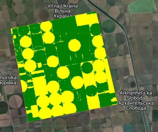

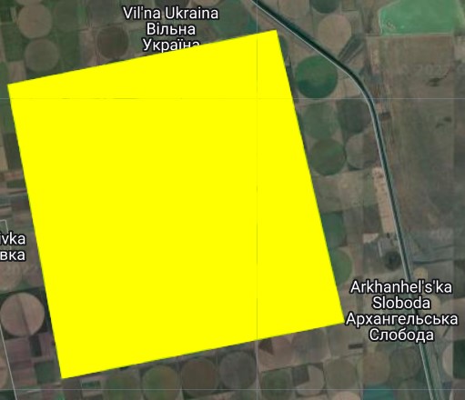
By toggling the canopy layers on and off superimposed over the ‘NDMI 2022’ and ‘Kakhovka 2022’ images, you will notice that brown areas correspond with low NDMI values, and are mostly the ones with a value 1 in the ‘No canopy’ image. The vice versa applies to areas in green. They have high NDMI values in the ‘NDMI 2022’ image and are those with value 1 (green) in the ‘Mid canopy’ image. It has also been noted that there were no crops that had high/total canopy cover or were waterlogged in this period. This explains why the ‘Very High Canopy’ image is all yellow (value 0).
Phase V: Interpreting the chart
Below are the charts for the NDMI image collection.
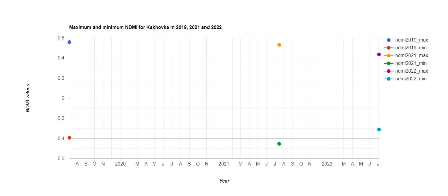
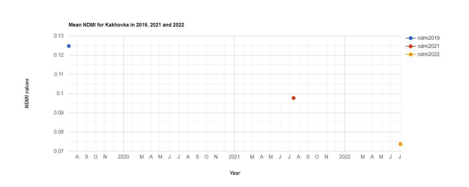
Even though the minimum NDMI for our AOI in 2022 was higher than for the preceding two years, its maximum and mean NDMI values are lower than for the previous years. Could the ongoing war have played a role in this?
Conclusion
NDMI is a good index to assess crop health, specifically water stress over an agricultural area. It is suitable for medium to large-sized crop fields and is helpful in identifying which farm areas are experiencing water stress and agricultural drought. The high resolution of Sentinel-2 images (10m), offers a much higher advantage in the assessment of moderately-sized farms compared to Landsat-8 or 9 which have coarser resolutions. Additionally, Sentinel-2 has a higher revisit time, 10-days to be exact, which allows near-seamless crop monitoring. This coupled with its free and open-source availability makes it a cheap and reliable source for water stress monitoring in moderate to large-sized farms.
Full code script for NDMI study over Kakhovka irrigation system
// get the coordinates for kakhovka irrigation system, Ukraine

Map.setCenter( 33.788277,  46.471417, 10);

// convert to satellite view to have a better understanding of
// kakhovka irrigation system

// add shapefile for Kakhosvka administration area extracted from this dataset
// https://data.humdata.org/dataset/cod-ab-ukr?

Map.addLayer(kakhovka_admin, {}, 'Kakhovka');

var irrigationArea = irrigation.area({'maxError': 1 }); // get area of selected agricultural block
print('Area of irrigated area: ', irrigationArea);

// there are some towns within the irrigation fields.
// we draw a region without towns and factories to avoid distortion of results

// we are going to use a pre-war image and a post war image to check ndmi of
// the irrigation system. Images will be in the month of July - least cloudy, hottest and least rainy.

// sentinel-2 image for 2019. Drought period
// load a sentinel-2 image over kakhovska in 2019
var kakh2019 = ee.ImageCollection('COPERNICUS/S2_SR')
     .filterBounds(irrigation)   // filter satellite images to those intersecting the irrigation area
     .filterDate('2019-07-01', '2019-07-30')  // fitler to month of July
     .sort('CLOUDY_PIXEL_PERCENTAGE')  // filter by cloud cover
     .first();               // choose least cloudy image

print('Kakhovka 2019', kakh2019);

var kakhovka2019 = kakh2019.clip(irrigation);

Map.addLayer(kakhovka2019, {bands: ['B4', 'B3', 'B2'], min:300, max: 6000},
'Kakhovka 2019');

Map.centerObject(kakhovka2019, 12);


// Sentinel-2 image for year 2021 (after cyclone)

var kakh2021 = ee.ImageCollection('COPERNICUS/S2_SR')
    .filterBounds(irrigation)
    .filterDate('2021-07-01', '2021-07-30')  // filter to 2021 image
    .sort('CLOUDY_PIXEL_PERCENTAGE')
    .first();

print('Kakhovka 2021', kakh2021);

var kakhovka2021 = kakh2021.clip(irrigation);

Map.addLayer(kakhovka2021, {bands: ['B4', 'B3', 'B2'], min:300, max: 6000},
'Kakhovka 2021');

// Sentinel-2 image for 2022 (after Russian invasion)

var kakh2022 = ee.ImageCollection('COPERNICUS/S2_SR')
    .filterBounds(irrigation)
    .filterDate('2022-07-01', '2022-07-30')  // filter to 2021 image
    .sort('CLOUDY_PIXEL_PERCENTAGE')
    .first();

print('Kakhovka 2022', kakh2022);

var kakhovka2022 = kakh2022.clip(irrigation);

Map.addLayer(kakhovka2022, {bands: ['B4', 'B3', 'B2'], min:300, max: 6000},
'Kakhovka 2022');

/////////////////////////////////////////////////////////////////////
/////////////////////////////////////////////////////////////////////


// calculate Normalized Difference Vegetation Index (NDMI)
// NDMI formula is NDMI = (NIR – SWIR) / (NIR + SWIR)
// ndmi formula using a Sentinel-2 image is NDMI = (B08 – B11)/(B08 + B11)

// NDMI for 2019
var ndmi2019 = kakhovka2019.normalizedDifference(['B8', 'B11'])
    .rename('ndmi2019');

// create a duplicate ndmi image with time data for original image copied.
// this will assist in creating the chart which requires time metadata
var NDMI2019 = ndmi2019.copyProperties(kakhovka2019, ['system:time_start']);

print('NDMI 2019', ndmi2019);
print('NDMI_2019', NDMI2019);


Map.addLayer(ndmi2019, {palette: ['red', 'yellow', 'green']}, 'NDMI 2019');
//Map.addLayer(NDMI2019, {palette: ['red', 'yellow', 'green']}, 'NDMI_2019');
// NDMI for 2021
var ndmi2021 = kakhovka2021.normalizedDifference(['B8', 'B11'])
    .rename('ndmi2021');

var NDMI2021 = ndmi2021.copyProperties(kakhovka2021, ['system:time_start']);
print('NDMI 2021', ndmi2021);
print('NDMI_2021', NDMI2021);

Map.addLayer(ndmi2021, {palette: ['red', 'yellow', 'green']}, 'NDMI 2021');

// NDMI for 2022
var ndmi2022 = kakhovka2022.normalizedDifference(['B8', 'B11'])
    .rename('ndmi2022');

var NDMI2022 = ndmi2022.copyProperties(kakhovka2022, ['system:time_start']);

print('NDMI 2022', ndmi2022);
print('NDMI_2022', NDMI2022);

Map.addLayer(ndmi2022, {palette: ['red', 'yellow', 'green']}, 'NDMI 2022');


// draw a chart showing the maximum ndmi over the years 2019, 2021 and 2022

// first convert our ndmi images of 2019, 2021 and 2022 into a collection
var col = ee.ImageCollection.fromImages([ndmi2019, ndmi2021, ndmi2022]);
print('NDMI Collection 2019 - 2022', col);

var col2 = ee.ImageCollection.fromImages([NDMI2019, NDMI2021, NDMI2022]);
print('NDMI Collection 2019 - 2022 with time properties', col2);

// set the chart style
var chartStyle = {
  title: 'Maximum and minimum NDMI for Kakhovka in 2019, 2021 and 2022',
  hAxis: {
    title: 'Year',
    titleTextStyle: {italic: true, bold: true}
  },
  vAxis: {
   title: 'NDMI values',
   titleTextStyle: {italic: true, bold: true},
   format: 'short'
  },
  pointSize: 10,

};

// draw the chart with max and min variation of NDMI values in 2019, 2021 and 2022
var chart_minmax = ui.Chart.image.series({
  imageCollection: col2,
  region: irrigation,
  reducer: ee.Reducer.minMax(),
  scale: 10,

});

chart_minmax.setOptions(chartStyle);

print('Chart for min-max NDMI', chart_minmax);

// draw the chart for the mean ndmi in 2019, 2021 and 2022

var chartStyle2 = {
  title: 'Mean NDMI for Kakhovka in 2019, 2021 and 2022',
  hAxis: {
    title: 'Year',
    titleTextStyle: {italic: true, bold: true}
  },
  vAxis: {
   title: 'NDMI values',
   titleTextStyle: {italic: true, bold: true},
   format: 'short'
  },
  pointSize: 10,

};


var chart_mean = ui.Chart.image.series({
  imageCollection: col2,
  region: irrigation,
  reducer: ee.Reducer.mean(),
  scale: 10,

});

chart_mean.setOptions(chartStyle2);

print('Chart for mean NDMI', chart_mean);


// extract the following values from 2022 image
// extract irrigation fields with 'almost absent' to 'Low canopy cover, Low canopy cover, low vigour or very low canopy cover, high vigour,'
var absentcanopy2022 = ndmi2022.expression(
  'band >= -1 and band <= 0', {
    'band': ndmi2022.select('ndmi2022')
  });

Map.addLayer(absentcanopy2022, {palette: ['yellow', 'green']}, 'No canopy');

// extract irrigation fields with 'mid-low canopy cover' to 'Mid-high canopy cover, low vigour or average canopy cover, high vigour'
var midcanopy2022 = ndmi2022.expression(
  'band > 0 and band <= 0.5', {
    'band': ndmi2022.select('ndmi2022')
  });

Map.addLayer(midcanopy2022, {palette: ['yellow', 'green']}, 'Mid high canopy');

// extract irrigation fields with very little canopy cover
var highcanopy2022 = ndmi2022.expression(
  'band >= 0.5 and band <= 1', {
    'band': ndmi2022.select('ndmi2022')
  });

Map.addLayer(highcanopy2022, {palette: ['yellow', 'green']}, 'Very high canopy');


Using the Normalized Difference Moisture Index