Speaking of high temperatures or land surface temperature estimations, our advanced spaceborne sensors have been collecting the earth’s thermal characteristics for decades. The new sensors such as Landsat 8, were launched to monitor these metrics even more accurately. The applications of the sensors span many sectors such as Precision Agriculture, Monitoring and Evaluation.
For the past few days, some hot news, and literally hot as an oven has been trending from China. Apparently, temperatures have been soaring high for the past weeks. In some places, the temperatures crossed the 35 degrees threshold, which is way above the recommended human comfort zone. There have been reports of roads buckling under the heat, melting of some roofs and heatstroke-related hospitalizations.
Heatwaves and searing summers are not uncommon in China. However, there are a couple of cities well known for their baking-hot temperatures that have earned the name ‘furnace cities’.
According to the ChinaHighlights, there are about ten cities famous, or infamous for their searing temperatures. They are Chongqing, Fuzhou, Hangzhou, Nanchang, Changsha, Wuhan, Xian, Nanjing, Hefei, and Nanning. The first three–Chongqing, Fuzhou and Hangzhou seem to be a tad above the rest and ironically, are situated close to mountains. It is actually in Chongqing that a roof of a restaurant popped out.
Land surface temperature estimations have been featured in a plethora of scientific studies and applications. Key among these is the study of climate change. For example, the prediction of El Nino Southern Oscillation (ENSO) is done by analyzing sea surface temperatures. Similarly, the prediction of weather hazards such as cyclones, and the validation of climatological studies, are all made possible using land and sea temperature records. The first use of satellites to measure the earth’s thermal characteristics dates back to the 1960s at the height of the Cold War. It was during this time that Nimbus, a satellite containing infrared measuring equipment, was launched and this opened the chapter of thermal sensing using remote sensing.
A particular satellite that has been used in numerous thermal measurements has been Landsat 8. Landsat 8 contains two thermal bands, Thermal Infrared 1 and Thermal Infrared 2, each with a 30m resolution. This makes it more reliable for thermal estimation compared to Sentinel 3 or MODIS which have higher spatial resolutions of up to 1km. Furthermore, innumerable studies have used Landsat missions for their terrestrial thermal assessments. We will simply ride on this advantage to conduct a Land Surface Temperature (LST) estimation over Chongqing. The image(s) to be used will be acquired from the July – September months, smack in the middle of the furnace season known for its sweltering heat. It will be noteworthy to mention July images for 2022 were currently unavailable, therefore we backtracked to 2021.
For this assessment, Google Earth Engine was used and data was acquired from Landsat 8. The main advantage of GEE is that it provides the user with server-based online computations, thus saving the user on storage and from intensive use of computer resources common in remote sensing tasks. Additionally, a tool with a wide user-community base comes with the advantage that there is always a high likelihood of some already designed free code for the exact task you had in mind. This not only saves time in that you won’t start from scratch but much-needed sanity is preserved especially when dealing with unintuitive programming language with a knack for throwing errors.
Below is the full script for estimating the land surface temperature for Chongqing city. The end goal was to create an image depicting the LST variation in the vicinity of Chongqing city. This would help us understand how physical and anthropogenic factors influence the LST of a region.
First, here is the code for the geometries used.
PS: The variables chongqing and aoi refer to the point and region of interest (ROI) geometries used in this study.
// Below is the JavaScript Code representing the current imports. To transfer them to another script, paste this code into the editor and click 'Convert' in the suggestion tooltip.

var chongqing = /* color: #d63000 */ee.Geometry.Point([106.49641035937503, 29.534924589334878]),
    aoi =
    /* color: #98ff00 */
    /* shown: false */
    /* displayProperties: [
      {
        "type": "rectangle"
      }
    ] */
    ee.Geometry.Polygon(
        [[[106.48349929062431, 29.684211326582403],
          [106.48349929062431, 28.876882759403152],
          [107.51346755234306, 28.876882759403152],
          [107.51346755234306, 29.684211326582403]]], null, false);
Here is the code for the Land Surface Temperature estimations
// get coordinates of Chongqing city

Map.setCenter(106.551342,  29.565687, 10);

//get least cloudy Landsat 8 raw image for Chongqing city for July

var landsat8 = ee.ImageCollection('LANDSAT/LC08/C02/T1')
    .filterDate('2021-07-01', '2021-10-30') //filtered date to the hottest period in Chongqing (july to august)
    .filterBounds(chongqing)  //filtered the images to within our location - chongqing
    .sort('CLOUD_COVER')    //sorted the image according to percentage cloud_cover in ascending order
    .first()         //chose the least cloudy image


// add landsat 8 layer to GEE
Map.addLayer(landsat8, {bands: ['B4', 'B3', 'B2'], min: 6000, max: 20000},
'Chongqing Landsat8');

//print results of the landsat 8 image over Chongqing
print('Chongqing L8 raw image: ', landsat8);

// clip the landsat 8 raw image to within the bounds of Chongqing
// since the landsat 8 raw image does not fully cover Chongqing
// the AoI shall extend to Fuling District, Nanchuan District, and Qijiang District

var AOI = landsat8.clip(aoi);

Map.addLayer(AOI, {bands: ['B4', 'B3', 'B2'], min: 6000, max: 20000},
'AOI');

// procedure for calculation of Land Surface Temperature (LST) was borrowed from --
//https://giscrack.com/how-to-calculate-land-surface-temperature-with-landsat-8-images/?utm_source=pocket_mylist

/// Step 1: Calibration of Landsat DN to TOA reflectance and Brightness temperature

// the conversation to brightness temperature which will be used afterwards
// can be automatically done with the ee.Algorithms.Landsat.TOA(input)

var BT = ee.Algorithms.Landsat.TOA(AOI);
var BT = BT.select('B10');
var BT = BT.rename('BT');

print('BT', BT);

Map.addLayer(BT, {}, 'BT');

/// Step 2: Calculate the NDVI
//NDVI is (NIR - R)/(NIR + R) or (B5 - B4)/(B5 + B4)

// can also use the ee.Image.normalizedDifference() function
var ndvi = AOI.normalizedDifference(['B5', 'B4']).rename('ndvi');

print('NDVI', ndvi);

Map.addLayer(ndvi, {palette: ['red', 'yellow', 'green'], min: -1, max: 1}, 'NDVI');

/// Step 3: Calculate the proportion of vegetation Pv

// Pv = Square ((NDVI – NDVImin) / (NDVImax – NDVImin))

// with gratitude to this stack overflow question
// https://gis.stackexchange.com/questions/306012/google-earth-engine-equation-for-fractional-vegetation-using-ndvi

// get maximum NDVI
var max = ee.Number(ndvi.reduceRegion({
  reducer: ee.Reducer.max(),
  geometry: aoi,
  scale: 30,
  bestEffort: true,
  maxPixels: 1e7
}).values().get(0));

print('Max NDVI:', max);

// get minimum NDVI
var min = ee.Number(ndvi.reduceRegion({
  reducer: ee.Reducer.min(),
  geometry: aoi,
  scale: 30,
  bestEffort: true,
  maxPixels: 1e7
}).values().get(0));

print('Min NDVI:', min);

var Pv = (ndvi.subtract(min).divide(max.subtract(min))).pow(ee.Number(2)).rename('Pv');

print('Proportion of Vegetation: ', Pv);

Map.addLayer(Pv, {palette: ['red', 'yellow', 'green']}, 'Proportion of Vegetation');

/// Step 4: Calculate emissivity

//ε = 0.004 * Pv + 0.986
var a = ee.Number(0.004);
var b = ee.Number(0.986);

var E = (Pv.multiply(a).add(b)).rename('Em');

print('Emissivity:', E);

Map.addLayer(E, {}, 'Emissivity');

/// Step 5: Calculate the land surface temperature

// The formula to calculate the land surface temperature is shown below:
// LST = (BT / (1 + (0.00115 * BT / 1.4388) * Ln(ε)))
// source: https://giscrack.com/how-to-calculate-land-surface-temperature-with-landsat-8-images/?utm_source=pocket_mylist

var LST = BT.expression(
  //LST = (BT / (1 + (0.00115 * BT / 1.4388) * Log(Ep)))
'(BT / (1 + (0.00115 * BT / 1.4388) * log(Ep))) - 273.15', {
 'BT': BT,
'Ep': E.select('Em')
}).rename('LST');

Map.addLayer(LST, {palette:['blue', 'yellow', 'red'], min: 18, max: 50}, 'Land Surface Temperature');

print('LST:', LST);

// get maximum values for Land Surface Temperature (LST)

var LST_max = ee.Number(LST.reduceRegion({
  reducer: ee.Reducer.max(),
  geometry: aoi,
  scale: 30,
  bestEffort: true,
  maxPixels: 1e7
}).values().get(0));

print('LST_Max', LST_max);

// get minimum values for Land Surface Temperature (LST)

var LST_min = ee.Number(LST.reduceRegion({
  reducer: ee.Reducer.min(),
  geometry: aoi,
  scale: 30,
  bestEffort: true,
  maxPixels: 1e7
}).values().get(0));

print('LST_Min', LST_min);

//Export the LST image
Export.image.toDrive({
  image: LST,
  description: 'land_surface_temperature',
  folder: 'test',
  region: aoi,
  scale: 30,
  fileFormat: 'GeoTIFF'
});
That’s a huge line of code. Leonardo Da Vinci said, “simplicity is the best sophistication”. The process of LST estimation looks and actually is complicated if the formulas from academic journals are anything to go by. However, and thanks to the help of GIS/RS enthusiasts such as GISCrack, the mathematical mumbo jumbo has been reduced to just six steps. With the help of the ee.Algorithms.Landsat.TOA(), it comes down to five. The drawback is, the 6 steps were done in ArcGIS, but doing the process in GEE is not so straightforward.
Secondly, most sat images over Chongqing had high cloud cover, obscuring the city and surrounding territory. Actually, the furnace season coincides with the most cloudy months. Therefore, to get at least one clear image was no walk in the park thus the backtracking to 2021.
Thirdly, the available 2021 image clipped out large areas towards the west of Chongqing. Nevertheless, a supplementary image showing the heat variation for these cut-out areas has been provided albeit it is from September–towards the tail end of the furnace season.
Step 1: Calibration of Landsat 8 DN to TOA reflectance and Brightness temperature
First things first. Satellites store the raw data they have collected in their bands in the form of Digital Numbers (DNs). These DNs are the corresponding pixels you see when you view an unprocessed image. Typically, DNs range in the values 0 – 255. This step is important in that it converts the values in the DNs to reflectance values. This is not only faithfully done by the ee.Algorithms.Landsat.TOA() algorithm, but they are also converted to brightness temperature (BT) as well. This, together with the emissivity are the two main ingredients for calculating LST.
Step 2: Calculate the NDVI
Where does NDVI come in all this mix? As a matter of fact, the values that will be got from NDVI will be used in calculating the emissivity, which will go in as one of the parameters to calculate LST. It is more like a cog in a wheel. The GISCrack team could not fit it any better in words: calculation of the NDVI is important because, subsequently, the proportion of vegetation (Pv), which is highly related to the NDVI, and emissivity (ε), which is related to the Pv, must be calculated.
Step 3: Calculate the proportion of vegetation Pv
Pv in very very very simple terms is the ratio of the vertical projection area of vegetation (leaves, stalks and branches) on the ground vis a vis the total vegetation area. In a more relatable way, it is like measuring the ratio of the height of buildings against the total area covered by the building (otherwise known as building footprint in construction lingo).
Step 4: Calculate Emissivity
Now we are getting closer to the goal. Emissivity is defined as the ratio of the energy radiated from a material’s surface to that radiated from a perfect emitter, known as a blackbody, at the same temperature and wavelength and under the same viewing conditions. Believe me, that’s the simplest definition that still pays respect to other physics principles. Our source also mentions that it is a … dimensionless number between 0 (for a perfect reflector) and 1 (for a perfect emitter).
Step 5: Calculate the Land Surface Temperature
Now to the grand finale. This stage marks the end of a strenuous process of understanding the concepts and calculations. If one has got the emissivity and brightness temperature conversion results all right, only one formula closes the chapter. Despite this safe arrival, the complicated nature of GEE Javascript language may soon turn short-lived relief into instant grief. For previous users of GEE, -, +, *, / and other mathematical operators are not recognised unless used in an expression. The same job is used with long-form methods of .multiply, .divide and likewise for +, -, and other mathematical operators. To bypass this pesky problem, the trick of encompassing all this into an expression, as used by Arya Danih was swiftly settled on. Riding on his ingenuity, our part only involved replacing the values used with those from our study.
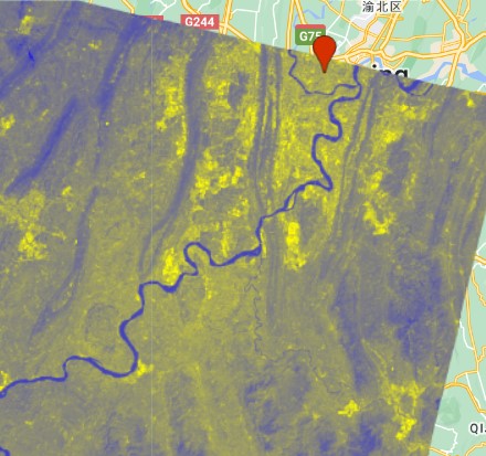
The following is the Land Surface Temperature map for Chongqing, 2nd August 2021.
For August 2021, the highest LST for our AOI was 50.7 degrees Celcius while the lowest was 18.2 degrees Celcius.
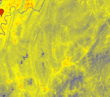
To cover the clipped region, an equally almost cloudless image was acquired. However, this image was for 26th September 2021, where the date is unfortunately at the tail-end of the furnace season. Nevertheless, it almost covers the entire Chongqing city.
The max and min LST values for Chongqing, in September 2021 were 42.4C and 17.8
C respectively.
In both images, it can be seen areas further away from the city core have lower LSTs compared to the city centre. For the August image, the LST difference between the city and urban fringe is more pronounced. It can be seen that the Chongqing city core and the CBDs of surrounding satellite centres have a tinge of red surrounded by a mix-mash of yellow and blue representing the suburbia and rural areas. The Yangtze river and the more vegetated and mountainous areas to the southeast are in blue indicating they have lower LST values. The blue patches to the South are clouds.
For the September image, the city core is in yellow and the surrounding areas with more vegetation are in blue indicating they have lower LSTs. In both images, the urban heat island is manifested.
Below is the temperature range for Chongqing city in 2021.

The daily range of reported temperatures (grey bars) and 24-hour highs (red ticks) and lows (blue ticks), placed over the daily average high (faint red line) and low (faint blue line) temperature, with 25th to 75th and 10th to 90th percentile bands.
Conclusion
According to the literature, large differences between satellite-derived LST and on-ground measurements can be large due to the resolution of the thermal band, NIR and Red bands (30m each) and other factors such as wind, humidity etc. Using the above weather chart for Chongqing in 2021 as our benchmark, highs (red ticks) and lows (blue ticks) for the first week of August 2021 were 34 degrees and 26 degrees. The same weather chart shows the last week of September had highs of 25 degrees and lows of 19 degrees, but in our September image, 42.4 degrees and 17.8 degrees are the extremes. Our image results may differ by and large, but if you consider that we covered a larger spatial area, and there are places in the chart which fell outside the red and blue lines–the ‘outliers’ with extreme highs and lows–then our image findings are within good ‘range’.
Code for the September image
// Below is the JavaScript Code representing the current imports. To transfer them to another script, paste this code into the editor and click 'Convert' in the suggestion tooltip.

var chongqing = /* color: #d63000 */ee.Geometry.Point([106.51426314257816, 29.58982746271335]),
    aoi =
    /* color: #98ff00 */
    /* shown: false */
    /* displayProperties: [
      {
        "type": "rectangle"
      }
    ] */
    ee.Geometry.Polygon(
        [[[105.85680260371332, 29.71801368474097],
          [105.85680260371332, 28.68470518903652],
          [106.84831871699457, 28.68470518903652],
          [106.84831871699457, 29.71801368474097]]], null, false);

// get coordinates of Chongqing city

Map.setCenter(106.551342,  29.565687, 10);

//get least cloudy Landsat 8 raw image for Chongqing city


var images = ee.ImageCollection('LANDSAT/LC08/C02/T1')
    .filterDate('2021-07-01', '2021-10-30') //filtered date to the hottest period in Chongqing (july to august)
    .filterBounds(chongqing)  //filtered the images to within our location - chongqing
    .sort('CLOUD_COVER')    //sorted the image according to percentage cloud_cover in ascending order
            //chose the least cloudy image

var landsat8 = ee.Image('LANDSAT/LC08/C02/T1/LC08_128040_20210926') // chose September image
// add landsat 8 layer to GEE
Map.addLayer(landsat8, {bands: ['B4', 'B3', 'B2'], min: 6000, max: 20000},
'Chongqing Landsat8');

//print results of the landsat 8 image over Chongqing
print('Chongqing L8 raw image: ', landsat8);

// clip the landsat 8 raw image to within the bounds of Chongqing
// since the landsat 8 raw image does not fully cover Chongqing
// the AoI shall extend to Fuling District, Nanchuan District, and Qijiang District


var AOI = landsat8.clip(aoi);

Map.addLayer(AOI, {bands: ['B4', 'B3', 'B2'], min: 6000, max: 20000},
'AOI');

// procedure for calculation of Land Surface Temperature (LST) was borrowed from --
//https://giscrack.com/how-to-calculate-land-surface-temperature-with-landsat-8-images/?utm_source=pocket_mylist

/// Step 1: Calibration of Landsat DN to TOA reflectance and Brightness temperature

// the conversation to brightness temperature which will be used afterwards
// can be automatically done with the ee.Algorithms.Landsat.TOA(input)

var BT = ee.Algorithms.Landsat.TOA(AOI);
var BT = BT.select('B10');
var BT = BT.rename('BT');

print('BT', BT);

Map.addLayer(BT, {}, 'BT');

/// Step 2: Calculate the NDVI
//NDVI is (NIR - R)/(NIR + R) or (B5 - B4)/(B5 + B4)

// can also use the ee.Image.normalizedDifference() function
var ndvi = AOI.normalizedDifference(['B5', 'B4']).rename('ndvi');

print('NDVI', ndvi);

Map.addLayer(ndvi, {palette: ['red', 'yellow', 'green'], min: -1, max: 1}, 'NDVI');

/// Step 3: Calculate the proportion of vegetation Pv

// Pv = Square ((NDVI – NDVImin) / (NDVImax – NDVImin))

// with gratitude to this stack overflow question
// https://gis.stackexchange.com/questions/306012/google-earth-engine-equation-for-fractional-vegetation-using-ndvi

// get maximum NDVI
var max = ee.Number(ndvi.reduceRegion({
  reducer: ee.Reducer.max(),
  geometry: aoi,
  scale: 30,
  bestEffort: true,
  maxPixels: 1e7
}).values().get(0));

print('Max NDVI:', max);

// get minimum NDVI
var min = ee.Number(ndvi.reduceRegion({
  reducer: ee.Reducer.min(),
  geometry: aoi,
  scale: 30,
  bestEffort: true,
  maxPixels: 1e7
}).values().get(0));

print('Min NDVI:', min);

var Pv = (ndvi.subtract(min).divide(max.subtract(min))).pow(ee.Number(2)).rename('Pv');

print('Proportion of Vegetation: ', Pv);

Map.addLayer(Pv, {palette: ['red', 'yellow', 'green']}, 'Proportion of Vegetation');

/// Step 4: Calculate emissivity

//ε = 0.004 * Pv + 0.986
var a = ee.Number(0.004);
var b = ee.Number(0.986);

var E = (Pv.multiply(a).add(b)).rename('Em');

print('Emissivity:', E);

Map.addLayer(E, {}, 'Emissivity');

/// Step 5: Calculate the land surface temperature

// The formula to calculate the land surface temperature is shown below:
// LST = (BT / (1 + (0.00115 * BT / 1.4388) * Ln(ε)))
// source: https://giscrack.com/how-to-calculate-land-surface-temperature-with-landsat-8-images/?utm_source=pocket_mylist

var LST = BT.expression(
  //LST = (BT / (1 + (0.00115 * BT / 1.4388) * Log(Ep)))
'(BT / (1 + (0.00115 * BT / 1.4388) * log(Ep))) - 273.15', {
 'BT': BT,
'Ep': E.select('Em')
}).rename('LST');

Map.addLayer(LST, {palette:['blue', 'yellow', 'red'], min: 18, max: 51}, 'Land Surface Temperature');

print('LST:', LST);

// get maximum values for Land Surface Temperature (LST)

var LST_max = ee.Number(LST.reduceRegion({
  reducer: ee.Reducer.max(),
  geometry: aoi,
  scale: 30,
  bestEffort: true,
  maxPixels: 1e7
}).values().get(0));

print('LST_Max', LST_max);

// get minimum values for Land Surface Temperature (LST)

var LST_min = ee.Number(LST.reduceRegion({
  reducer: ee.Reducer.min(),
  geometry: aoi,
  scale: 30,
  bestEffort: true,
  maxPixels: 1e7
}).values().get(0));

print('LST_Min', LST_min);

//Export the LST image
Export.image.toDrive({
  image: LST,
  description: 'land_surface_temperature',
  folder: 'test',
  region: aoi,
  scale: 30,
  fileFormat: 'GeoTIFF'
});
Landsat 8 in Land Surface Temperature Estimations